Preface
Copyright Mark Watson. All rights reserved. This book may be shared using the Creative Commons “share and share alike, no modifications, no commercial reuse” license.
The latest edition of this book is always available at https://leanpub.com/javaai. You can also download a free copy from my website. Currently the latest edition was released in the summer of 2020. It had been seven years since the previous edition and this is largely a rewrite, dropping some material like Drools based expert systems, Weka for machine learning, and the implementation of an RDF server with geolocation support. I am now placing a heavier emphasis on neural networks and deep learning, a greatly expanded discussion of the semantic web and linked data including examples to generate knowledge graphs automatically from text documents and also a system to help navigate public Knowledge Graphs like DBPedia and WikiData.
The code and PDF for the 4th edition from 2013 can be found here.
I decided which material to keep from old editions and which new material to add based on what my estimation is of which AI technologies are most useful and interesting to Java developers.
I have been developing commercial Artificial Intelligence (AI) tools and applications since the 1980s.

I wrote this book for both professional programmers and home hobbyists who already know how to program in Java and who want to learn practical AI programming and information processing techniques. I have tried to make this an enjoyable book to work through. In the style of a “cook book,” the chapters can be studied in any order. When an example depends on a library developed in a previous chapter this is stated clearly. Most chapters follow the same pattern: a motivation for learning a technique, some theory for the technique, and a Java example program that you can experiment with.
The code for the example programs is available on github:
https://github.com/mark-watson/Java-AI-Book-Code
My Java code in this book can be used under either or both the LGPL3 and Apache 2 licenses - choose whichever of these two licenses that works best for you. Git pull requests with code improvements will be appreciated by me and the readers of this book.
My goal is to introduce you to common AI techniques and to provide you with Java source code to save you some time and effort. Even though I have worked almost exclusively in the field of deep learning in the last six years, I urge you, dear reader, to look at the field of AI as being far broader than machine learning and deep learning in particular. Just as it is wrong to consider the higher level fields of Category Theory or Group Theory to “be” mathematics, there is far more to AI than machine learning. Here we will take a more balanced view of AI, and indeed, my own current research is in hybrid AI, that is, the fusion of deep learning with good old fashioned symbolic AI, probabilistic reasoning, and explainability.
This book is released with a Attribution-NonCommercial-NoDerivatives 4.0 International (CC BY-NC-ND 4.0) license. Feel free to share copies of this book with friends and colleagues at work. This book is also available to read free online or to purchase if you want to support my writing activities.
Personal Artificial Intelligence Journey
I have been interested in AI since reading Bertram Raphael’s excellent book Thinking Computer: Mind Inside Matter in the early 1980s. I have also had the good fortune to work on many interesting AI projects including the development of commercial expert system tools for the Xerox LISP machines and the Apple Macintosh, development of commercial neural network tools, application of natural language and expert systems technology, medical information systems, application of AI technologies to Nintendo and PC video games, and the application of AI technologies to the financial markets. I have also applied statistical natural language processing techniques to analyzing social media data from Twitter and Facebook. I worked at Google on their Knowledge Graph and I managed a deep learning team at Capital One.
I enjoy AI programming, and hopefully this enthusiasm will also infect you, the reader.
Maven Setup for Combining Examples in this Book
The chapter on WordNet uses the examples from the previous chapter on OpenNLP. Both chapters discuss the use of maven to support this code and data sharing.
Additionally, the chapter Statistical Natural Language Processing is configured so the code and linguistic data can be combined with other examples.
Code sharing is achieved by installing the code in your local maven repository, for example:
1     cd Java-AI-Book-Code/opennlp
2     mvn install
Now, the code in the OpenNLP example is installed on your system.
Software Licenses for Example Programs in this Book
My example programs (i.e., the code I wrote) are licensed under the LGPL version 3 and the Apache 2. Use whichever of these two licenses that works better for you. I also use several open source libraries in the book examples and their licenses are:
- PowerLoom Reasoning: LGPL
- Jena Semantic Web: Apache 2
- OpenNlp: Apache 2
- WordNet: MIT style license (link to license)
- Deep Learning for Java (DL4J): Apache 2
My desire is for you to be able to use my code examples and data in your projects with no hassles.
Acknowledgements
I process the manuscript for this book using the leanpub.com publishing system and I recommend leanpub.com to other authors. Write one manuscript and use leanpub.com to generate assets for PDF, iPad/iPhone, and Kindle versions. It is also simple to push new book updates to readers.
I would like to thank Kevin Knight for writing a flexible framework for game search algorithms in Common LISP (Rich, Knight 1991) and for giving me permission to reuse his framework, rewritten in Java for some of the examples in the Chapter on Search. I would like to thank my friend Tom Munnecke for my photo in this Preface. I have a library full of books on AI and I would like to thank the authors of all of these books for their influence on my professional life. I frequently reference books in the text that have been especially useful to me and that I recommend to my readers.
In particular, I would like to thank the authors of the following two books that have probably had the most influence on me:
- Stuart Russell and Peter Norvig’s Artificial Intelligence: A Modern Approach which I consider to be the best single reference book for AI theory
- John Sowa’s book Knowledge Representation is a resource that I turn to for a holistic treatment of logic, philosophy, and knowledge representation in general
Book Editor: Carol Watson
Thanks to the following people who found typos in this and earlier book editions: Carol Watson, James Fysh, Joshua Cranmer, Jack Marsh, Jeremy Burt, Jean-Marc Vanel
Search
Unless you write the AI for game programs and entertainment systems (which I have done for Angel Studios, Nintendo, and Disney), the material in the chapter may not be relevant to your work. That said I recommend that you develop some knowledge of defining search spaces for problems and techniques to search these spaces. I hope that you have fun with the material in this chapter.
Early AI research emphasized the optimization of search algorithms. At this time in the 1950s and 1960s this approach made sense because many AI tasks can be solved effectively by defining state spaces and using search algorithms to define and explore search trees in this state space. This approach for AI research encountered some early success in game playing systems like checkers and chess which reinforced confidence in viewing many AI problems as search problems.
I now consider this form of classic search to be a well understood problem but that does not mean that we will not see exciting improvements in search algorithms in the future. This book does not cover Monte Carlo Search or game search using Reinforcement Learning with Monte Carlo Search that Alpha Go uses.
We will cover depth-first and breadth-first search. The basic implementation for depth-first and breadth-first search is the same with one key difference. When searching from any location in state space we start by calculating nearby locations that can be moved to in one search cycle. For depth-first search we store new locations to be searched in a stack data structure and for breadth-first search we store new locations to search in a queue data structure. As we will shortly see this simple change has a large impact on search quality (usually breadth-first search will produce better results) and computational resources (depth-first search requires less storage).
It is customary to cover search in AI books but to be honest I have only used search techniques in one interactive planning system in the 1980s and much later while doing the “game AI” in two Nintendo games, a PC hovercraft racing game and a VR system for Disney. Still, you should understand how to optimize search.
What are the limitations of search? Early on, success in applying search to problems like checkers and chess misled early researchers into underestimating the extreme difficulty of writing software that performs tasks in domains that require general world knowledge or deal with complex and changing environments. These types of problems usually require the understanding and the implementation of domain specific knowledge.
In this chapter, we will use three search problem domains for studying search algorithms: path finding in a maze, path finding in a graph, and alpha-beta search in the games tic-tac-toe and chess.
If you want to try the examples before we proceed to the implementation then you can do that right now using the Makefile in the search directory:
chess:
	mvn install
	mvn exec:java -Dexec.mainClass="search.game.Chess"

graph:
	mvn install
	mvn exec:java -Dexec.mainClass="search.graph.GraphDepthFirstSearch"

maze:
	mvn install
	mvn exec:java -Dexec.mainClass="search.maze.MazeBreadthFirstSearch"
You can run the examples using:
Representation of Search State Space and Search Operators
We will use a single search tree representation in graph search and maze search examples in this chapter. Search trees consist of nodes that define locations in state space and links to other nodes. For some small problems, the search tree can be pre-computed and cover all of the search space. For most problems however it is impossible to completely enumerate a search tree for a state space so we must define successor node search operators that for a given node produce all nodes that can be reached from the current node in one step. For example, in the game of chess we can not possibly enumerate the search tree for all possible games of chess, so we define a successor node search operator that given a board position (represented by a node in the search tree) calculates all possible moves for either the white or black pieces. The possible Chess moves are calculated by a successor node search operator and are represented by newly calculated nodes that are linked to the previous node. Note that even when it is simple to fully enumerate a search tree, as in the small maze example, we still want to use the general implementation strategy of generating the search tree dynamically as we will do in this chapter.
For calculating a search tree we use a graph. We will represent graphs as nodes with links between some of the nodes. For solving puzzles and for game related search, we will represent positions in the search space with Java objects called nodes. Nodes contain arrays of references to child nodes and for some applications we also might store links back to parent nodes. A search space using this node representation can be viewed as a directed graph or a tree. The node that has no parent nodes is the root node and all nodes that have no child nodes a called leaf nodes.
Search operators are used to move from one point in the search space to another. We deal with quantized search spaces in this chapter, but search spaces can also be continuous in some applications (e.g., a robot’s position while moving in the real world). In general search spaces are either very large or are infinite. We implicitly define a search space using some algorithm for extending the space from our reference position in the space. The figure Search Space Representations shows representations of search space as both connected nodes in a graph and as a two-dimensional grid with arrows indicating possible movement from a reference point denoted by R.
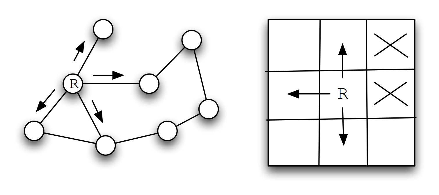
When we specify a search space as a two-dimensional array, search operators will move the point of reference in the search space from a specific grid location to an adjoining grid location. For some applications, search operators are limited to moving up/down/left/right and in other applications operators can additionally move the reference location diagonally.
When we specify a search space using node representation, search operators can move the reference point down to any child node or up to the parent node. For search spaces that are represented implicitly, search operators are also responsible for determining legal child nodes, if any, from the reference point.
Note that I created different libraries for the maze and graph search examples.
Finding Paths in Mazes
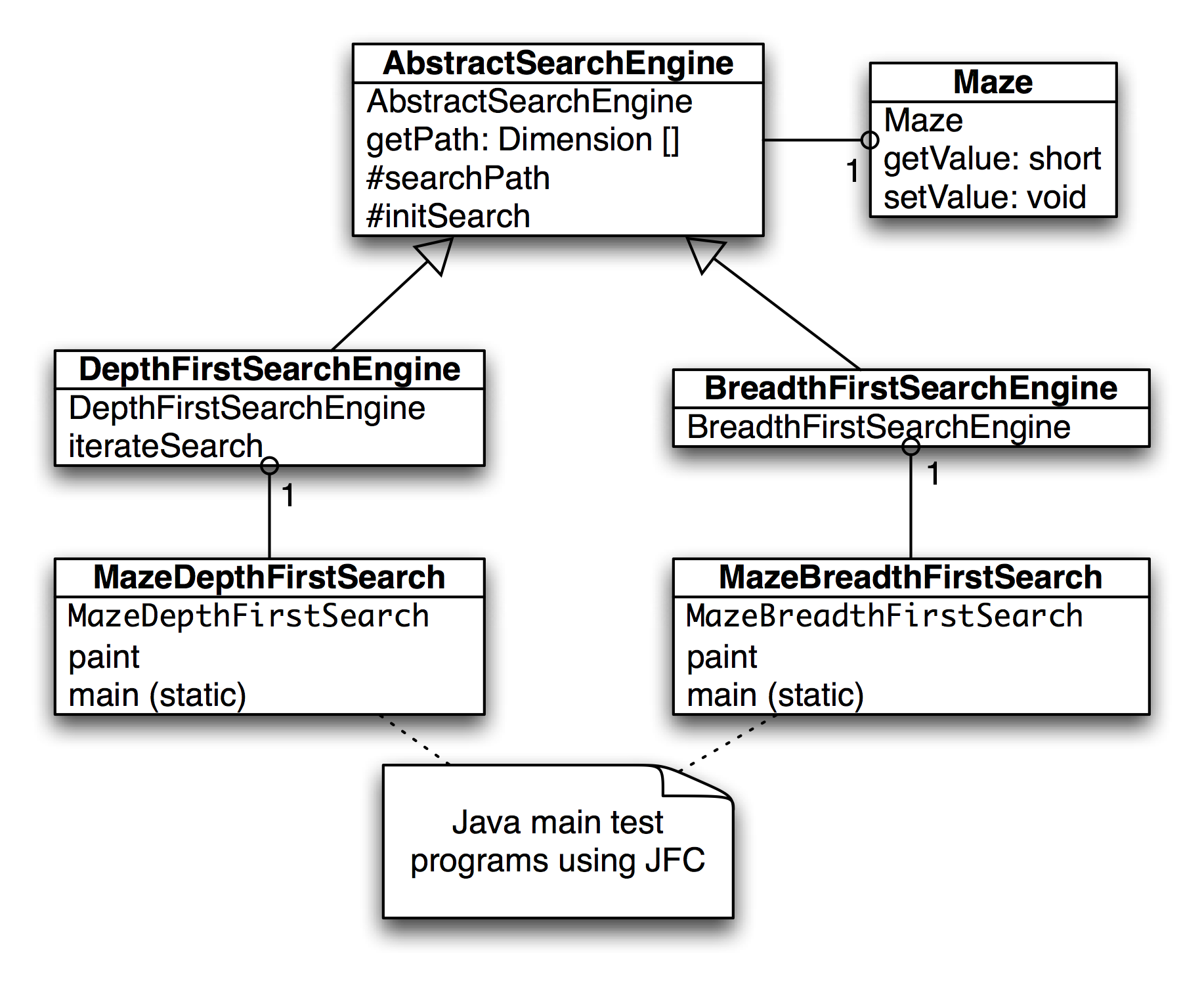
The example program used in this section is MazeSearch.java in the directory search/src/main/java/search/maze and I assume that you have cloned the GitHub repository for this book. The figure UML Diagram for Search Classes shows an overview of the maze search strategies: depth-first and breadth-first search. The abstract base class AbstractSearchEngine contains common code and data that is required by both the classes DepthFirstSearch and BreadthFirstSearch. The class Maze is used to record the data for a two-dimensional maze, including which grid locations contain walls or obstacles. The class Maze defines three static short integer values used to indicate obstacles, the starting location, and the ending location.
The Java class Maze defines the search space. This class allocates a two-dimensional array of short integers to represent the state of any grid location in the maze. Whenever we need to store a pair of integers, we will use an instance of the standard Java class java.awt.Dimension, which has two integer data components: width and height. Whenever we need to store an x-y grid location, we create a new Dimension object (if required), and store the x coordinate in Dimension.width and the y coordinate in Dimension.height. As in the right-hand side of figure Search Space, the operator for moving through the search space from given x-y coordinates allows a transition to any adjacent grid location that is empty. The Maze class also contains the x-y location for the starting location (startLoc) and goal location (goalLoc). Note that for these examples, the class Maze sets the starting location to grid coordinates 0-0 (upper left corner of the maze in the figures to follow) and the goal node in (width - 1) - (height - 1) (lower right corner in the following figures).
The abstract class AbstractSearchEngine is the base class for both the depth-first (uses a stack to store moves) search class DepthFirstSearchEngine and the breadth-first (uses a queue to store moves) search class BreadthFirstSearchEngine. We will start by looking at the common data and behavior defined in AbstractSearchEngine. The class constructor has two required arguments: the width and height of the maze, measured in grid cells. The constructor defines an instance of the Maze class of the desired size and then calls the utility method initSearch to allocate an array searchPath of Dimension objects, which will be used to record the path traversed through the maze. The abstract base class also defines other utility methods:
- equals(Dimension d1, Dimension d2) – checks to see if two arguments of type Dimension are the same.
- getPossibleMoves(Dimension location) – returns an array of Dimension objects that can be moved to from the specified location. This implements the movement operator.
Now, we will look at the depth-first search procedure. The constructor for the derived class DepthFirstSearchEngine calls the base class constructor and then solves the search problem by calling the method iterateSearch. We will look at this method in some detail. The arguments to iterateSearch specify the current location and the current search depth:
private void iterateSearch(Dimension loc, int depth) {
The class variable isSearching is used to halt search, avoiding more solutions, once one path to the goal is found.
if (isSearching == false) return;
We set the maze value to the depth for display purposes only:
maze.setValue(loc.width, loc.height, (short)depth);
Here, we use the super class getPossibleMoves method to get an array of possible neighboring squares that we could move to; we then loop over the four possible moves (a null value in the array indicates an illegal move):
      Dimension [] moves = getPossibleMoves(loc);
      for (int i=0; i<4; i++) {
        if (moves[i] == null) break; // out of possible moves
                                     // from this location
Record the next move in the search path array and check to see if we are done:
      searchPath[depth] = moves[i];
      if (equals(moves[i], goalLoc)) {
         System.out.println("Found the goal at " +
                            moves[i].width +
                            ``, " + moves[i].height);
         isSearching = false;
         maxDepth = depth;
         return;
      } else {
If the next possible move is not the goal move, we recursively call the iterateSearch method again, but starting from this new location and increasing the depth counter by one:
        iterateSearch(moves[i], depth + 1);
        if (isSearching == false) return;
      }
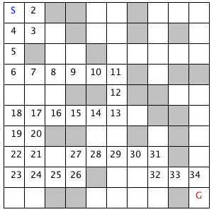
The figure showing the depth-first search in a maze shows how poor a path a depth-first search can find between the start and goal locations in the maze. The maze is a 10-by-10 grid. The letter S marks the starting location in the upper left corner and the goal position is marked with a G in the lower right corner of the grid. Blocked grid cells are painted light gray. The basic problem with the depth-first search is that the search engine will often start searching in a bad direction, but still find a path eventually, even given a poor start. The advantage of a depth-first search over a breadth-first search is that the depth-first search requires much less memory. We will see that possible moves for depth-first search are stored on a stack (last in, first out data structure) and possible moves for a breadth-first search are stored in a queue (first in, first out data structure).
The derived class BreadthFirstSearch is similar to the DepthFirstSearch procedure with one major difference: from a specified search location we calculate all possible moves, and make one possible trial move at a time. We use a queue data structure for storing possible moves, placing possible moves on the back of the queue as they are calculated, and pulling test moves from the front of the queue. The effect of a breadth-first search is that it “fans out” uniformly from the starting node until the goal node is found.
The class constructor for BreadthFirstSearch calls the super class constructor to initialize the maze, and then uses the auxiliary method doSearchOn2Dgrid for performing a breadth-first search for the goal. We will look at the class BreadthFirstSearch in some detail. Breadth first search uses a queue instead of a stack (depth-first search) to store possible moves. The utility class DimensionQueue implements a standard queue data structure that handles instances of the class Dimension.
The method doSearchOn2Dgrid is not recursive, it uses a loop to add new search positions to the end of an instance of class DimensionQueue and to remove and test new locations from the front of the queue. The two-dimensional array allReadyVisited keeps us from searching the same location twice. To calculate the shortest path after the goal is found, we use the predecessor array:
        private void doSearchOn2DGrid() {
          int width = maze.getWidth();
          int height = maze.getHeight();
          boolean alReadyVisitedFlag[][] =
                  new boolean[width][height];
          Dimension predecessor[][] =
                new Dimension[width][height];
          DimensionQueue queue =
                        new DimensionQueue();
          for (int i=0; i<width; i++) {
            for (int j=0; j<height; j++) {
              alReadyVisitedFlag[i][j] = false;
              predecessor[i][j] = null;
            }
          }
We start the search by setting the already visited flag for the starting location to true value and adding the starting location to the back of the queue:
          alReadyVisitedFlag[startLoc.width][startLoc.height]
             = true;
          queue.addToBackOfQueue(startLoc);
          boolean success = false;
This outer loop runs until either the queue is empty or the goal is found:
        outer:
          while (queue.isEmpty() == false) {
We peek at the Dimension object at the front of the queue (but do not remove it) and get the adjacent locations to the current position in the maze:
            Dimension head = queue.peekAtFrontOfQueue();
            Dimension [] connected =
                             getPossibleMoves(head);
We loop over each possible move; if the possible move is valid (i.e., not null) and if we have not already visited the possible move location, then we add the possible move to the back of the queue and set the predecessor array for the new location to the last square visited (head is the value from the front of the queue). If we find the goal, break out of the loop:
            for (int i=0; i<4; i++) {
              if (connected[i] == null) break;
              int w = connected[i].width;
              int h = connected[i].height;
              if (alReadyVisitedFlag[w][h] == false) {
                alReadyVisitedFlag[w][h] = true;
                predecessor[w][h] = head;
                queue.addToBackOfQueue(connected[i]);
                if (equals(connected[i], goalLoc)) {
                  success = true;
                  break outer; // we are done
                }
              }
            }
We have processed the location at the front of the queue (in the variable head), so remove it:
            queue.removeFromFrontOfQueue();
          }
Now that we are out of the main loop, we need to use the predecessor array to get the shortest path. Note that we fill in the searchPath array in reverse order, starting with the goal location:
          maxDepth = 0;
          if (success) {
            searchPath[maxDepth++] = goalLoc;
            for (int i=0; i<100; i++) {
              searchPath[maxDepth] =
                 predecessor[searchPath[maxDepth - 1].
                   width][searchPath[maxDepth - 1].
                   height];
              maxDepth++;
              if (equals(searchPath[maxDepth - 1],
                         startLoc))
                break;  // back to starting node
            }
          }
        }
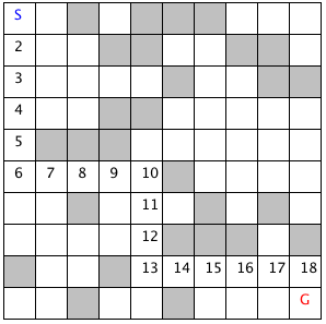
The figure of breadth search of a maze shows a good path solution between starting and goal nodes. Starting from the initial position, the breadth-first search engine adds all possible moves to the back of a queue data structure. For each possible move added to this queue in one search cycle, all possible moves are added to the queue for each new move recorded. Visually, think of possible moves added to the queue as “fanning out” like a wave from the starting location. The breadth-first search engine stops when this “wave” reaches the goal location. In general, I prefer breadth-first search techniques to depth-first search techniques when memory storage for the queue used in the search process is not an issue. In general, the memory requirements for performing depth-first search is much less than breadth-first search.
Note that the classes MazeDepthFirstSearch and MazeBreadthFirstSearch are simple Java JFC applications that produced the figure showing the depth-first search in a maze and the figure of breadth search of a maze. The interested reader can read through the source code for the GUI test programs, but we will only cover the core AI code in this book. If you are interested in the GUI test programs and you are not familiar with the Java JFC (or Swing) classes, there are several good tutorials on JFC programming on the web.
Finding Paths in Graphs
In the last section, we used both depth-first and breadth-first search techniques to find a path between a starting location and a goal location in a maze. Another common type of search space is represented by a graph. A graph is a set of nodes and links. We characterize nodes as containing the following data:
- A name and/or other data
- Zero or more links to other nodes
- A position in space (this is optional, usually for display or visualization purposes)
Links between nodes are often called edges. The algorithms used for finding paths in graphs are very similar to finding paths in a two-dimensional maze. The primary difference is the operators that allow us to move from one node to another. In the last section we saw that in a maze, an agent can move from one grid space to another if the target space is empty. For graph search, a movement operator allows movement to another node if there is a link to the target node.
The figure showing UML Diagram for Search Classes shows the UML class diagram for the graph search Java classes that we will use in this section. The abstract class AbstractGraphSearch class is the base class for both DepthFirstSearch and BreadthFirstSearch. The classes GraphDepthFirstSearch and GraphBreadthFirstSearch and test programs also provide a Java Foundation Class (JFC) or Swing based user interface. These two test programs produced figures Search Depth-First and Search Breadth-First.
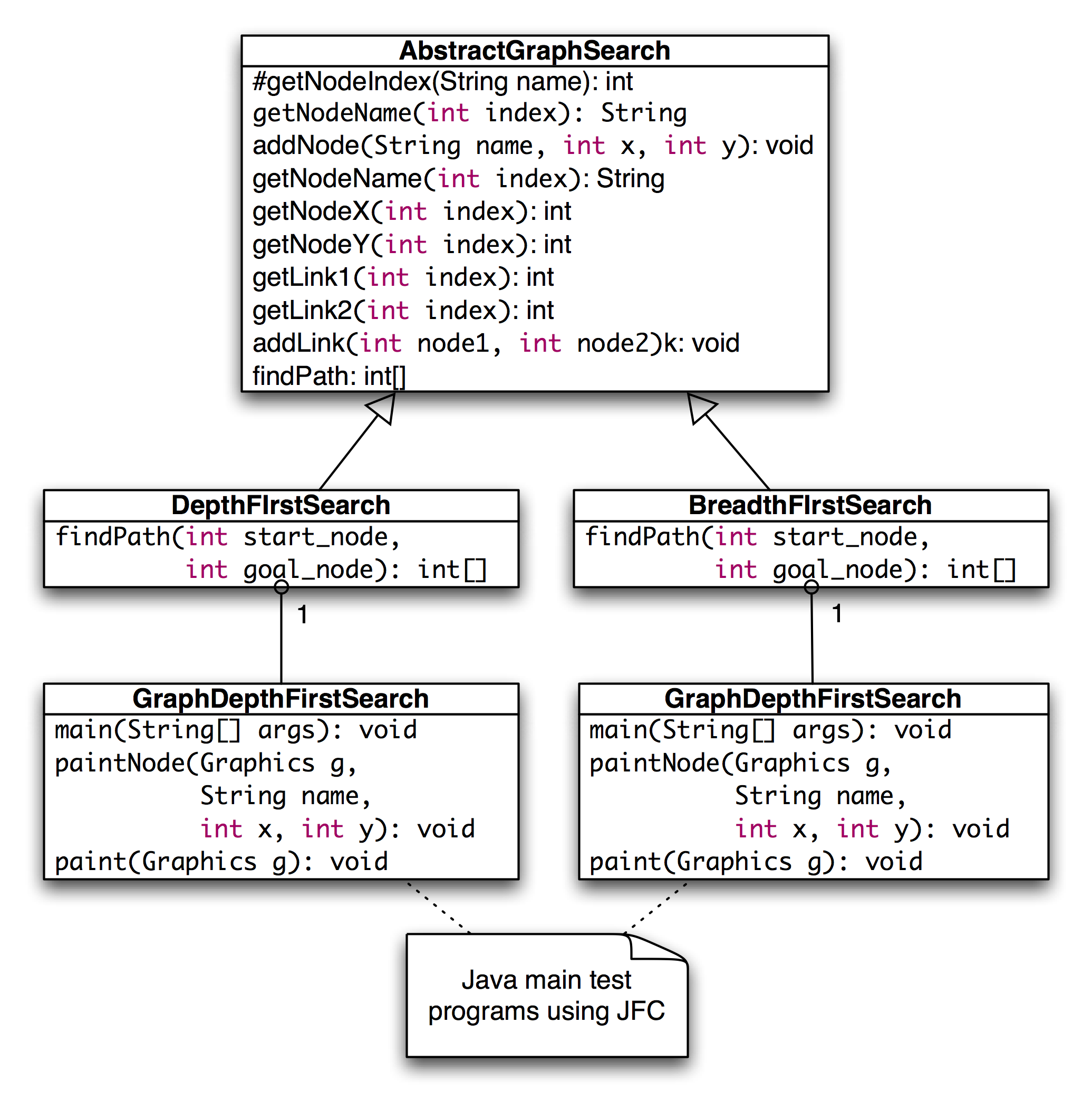
As seen in the previous figure, most of the data for the search operations (i.e., nodes, links, etc.) is defined in the abstract class AbstractGraphSearch. This abstract class is customized through inheritance to use a stack for storing possible moves (i.e., the array path) for depth-first search and a queue for breadth-first search.
The abstract class AbstractGraphSearch allocates data required by both derived classes:
        final public static int MAX = 50;
        protected int [] path =
              new int[AbstractGraphSearch.MAX];
        protected int num_path = 0;
        // for nodes:
        protected String [] nodeNames =
                               new String[MAX];
        protected int [] node_x = new int[MAX];
        protected int [] node_y = new int[MAX];
        // for links between nodes:
        protected int [] link_1 = new int[MAX];
        protected int [] link_2 = new int[MAX];
        protected int [] lengths = new int[MAX];
        protected int numNodes = 0;
        protected int numLinks = 0;
        protected int goalNodeIndex = -1,
                      startNodeIndex = -1;
The abstract base class also provides several common utility methods:
- addNode(String name, int x, int y) – adds a new node
- addLink(int n1, int n2) – adds a bidirectional link between nodes indexed by n1 and n2. Node indexes start at zero and are in the order of calling addNode.
- addLink(String n1, String n2) – adds a bidirectional link between nodes specified by their names
- getNumNodes() – returns the number of nodes
- getNumLinks() – returns the number of links
- getNodeName(int index) – returns a node’s name
- getNodeX(), getNodeY() – return the coordinates of a node
- getNodeIndex(String name) – gets the index of a node, given its name
The abstract base class defines an abstract method findPath that must be overridden. We will start with the derived class DepthFirstSearch, looking at its implementation of findPath. The findPath method returns an array of node indices indicating the calculated path:
      public int [] findPath(int start_node,
                             int goal_node) {
The class variable path is an array that is used for temporary storage; we set the first element to the starting node index, and call the utility method findPathHelper:
        path[0] = start_node; // the starting node
        return findPathHelper(path, 1, goal_node);
      }
The method findPathHelper is the interesting method in this class that actually performs the depth-first search; we will look at it in some detail:
The path array is used as a stack to keep track of which nodes are being visited during the search. The argument num_path is the number of locations in the path, which is also the search depth:
      public int [] findPathHelper(int [] path,
                                   int num_path,
                                   int goal_node) {
First, re-check to see if we have reached the goal node; if we have, make a new array of the current size and copy the path into it. This new array is returned as the value of the method:
        if (goal_node == path[num_path - 1]) {
          int [] ret = new int[num_path];
          for (int i=0; i<num_path; i++) {
             ret[i] = path[i];
          }
          return ret;  // we are done!
        }
We have not found the goal node, so call the method connected_nodes to find all nodes connected to the current node that are not already on the search path (see the source code for the implementation of connected_nodes):
        int [] new_nodes = connected_nodes(path,
                                           num_path);
If there are still connected nodes to search, add the next possible “node to visit” to the top of the stack (variable path in the program) and recursively call the method findPathHelper again:
        if (new_nodes != null) {
          for (int j=0; j<new_nodes.length; j++) {
            path[num_path] = new_nodes[j];
            int [] test = findPathHelper(new_path,
                                         num_path + 1,
                                         goal_node);
            if (test != null) {
              if (test[test.length-1] == goal_node) {
                  return test;
              }
            }
          }
        }
If we have not found the goal node, return null, instead of an array of node indices:
        return null;
      }
Derived class BreadthFirstSearch also must define abstract method findPath. This method is very similar to the breadth-first search method used for finding a path in a maze: a queue is used to store possible moves. For a maze, we used a queue class that stored instances of the class Dimension, so for this problem, the queue only needs to store integer node indices. The return value of findPath is an array of node indices that make up the path from the starting node to the goal.
      public int [] findPath(int start_node,
                             int goal_node) {
We start by setting up a flag array alreadyVisited to prevent visiting the same node twice, and allocating a predecessors array that we will use to find the shortest path once the goal is reached:
        // data structures for depth-first search:
        boolean [] alreadyVisitedFlag =
                               new boolean[numNodes];
        int [] predecessor = new int[numNodes];
The class IntQueue is a private class defined in the file BreadthFirstSearch.java; it implements a standard queue:
IntQueue queue = new IntQueue(numNodes + 2);
Before the main loop, we need to initialize the already visited predecessor arrays, set the visited flag for the starting node to true, and add the starting node index to the back of the queue:
        for (int i=0; i<numNodes; i++) {
          alreadyVisitedFlag[i] = false;
          predecessor[i] = -1;
        }
        alreadyVisitedFlag[start_node] = true;
        queue.addToBackOfQueue(start_node);
The main loop runs until we find the goal node or the search queue is empty:
outer: while (queue.isEmpty() == false) {
We will read (without removing) the node index at the front of the queue and calculate the nodes that are connected to the current node (but not already on the visited list) using the connected_nodes method (the interested reader can see the implementation in the source code for this class):
          int head = queue.peekAtFrontOfQueue();
          int [] connected = connected_nodes(head);
          if (connected != null) {
If each node connected by a link to the current node has not already been visited, set the predecessor array and add the new node index to the back of the search queue; we stop if the goal is found:
          for (int i=0; i<connected.length; i++) {
             if (alreadyVisitedFlag[connected[i]] == false) {
               predecessor[connected[i]] = head;
               queue.addToBackOfQueue(connected[i]);
               if (connected[i] == goal_node) break outer;
              }
            }
            alreadyVisitedFlag[head] = true;
            queue.removeFromQueue(); // ignore return value
          }
        }
Now that the goal node has been found, we can build a new array of returned node indices for the calculated path using the predecessor array:
        int [] ret = new int[numNodes + 1];
        int count = 0;
        ret[count++] = goal_node;
        for (int i=0; i<numNodes; i++) {
          ret[count] = predecessor[ret[count - 1]];
          count++;
          if (ret[count - 1] == start_node)  break;
        }
        int [] ret2 = new int[count];
        for (int i=0; i<count; i++) {
          ret2[i] = ret[count - 1 - i];
        }
        return ret2;
       }
In order to run both the depth-first and breadth-first graph search examples, change directory to src-search-maze and type the following commands:
    javac *.java
    java GraphDepthFirstSearch
    java GraphBeadthFirstSearch
The following figure shows the results of finding a route from node 1 to node 9 in the small test graph. Like the depth-first results seen in the maze search, this path is not optimal.
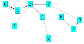
The next figure shows an optimal path found using a breadth-first search. As we saw in the maze search example, we find optimal solutions using breadth-first search at the cost of extra memory required for the breadth-first search.

Adding Heuristics to Breadth-first Search
We can usually make breadth-first search more efficient by ordering the search order for all branches from a given position in the search space. For example, when adding new nodes from a specified reference point in the search space, we might want to add nodes to the search queue first that are “in the direction” of the goal location: in a two-dimensional search like our maze search, we might want to search connected grid cells first that were closest to the goal grid space. In this case, pre-sorting nodes (in order of closest distance to the goal) added to the breadth-first search queue could have a dramatic effect on search efficiency. The alpha-beta additions to breadth-first search are seen in in the next section.
Heuristic Search and Game Playing: Tic-Tac-Toe and Chess
Now that a computer program has won a match against the human world champion, perhaps people’s expectations of AI systems will be prematurely optimistic. Game search techniques are not real AI, but rather, standard programming techniques. A better platform for doing AI research is the game of Go. There are so many possible moves in the game of Go that brute force look ahead (as is used in Chess playing programs) simply does not work. In 2016 the Alpha Go program became stronger than human players by using Reinforcement Learning and Monte Carlo search.
Min-max type search algorithms with alpha-beta cutoff optimizations are an important programming technique and will be covered in some detail in the remainder of this chapter. We will design an abstract Java class library for implementing alpha-beta enhanced min-max search, and then use this framework to write programs to play tic-tac-toe and chess.
Alpha-Beta Search
The first game that we will implement will be tic-tac-toe, so we will use this simple game to explain how the min-max search (with alpha-beta cutoffs) works.
The figure showing possible moves for tic-tac-toe shows some of the possible moves generated from a tic-tac-toe position where X has made three moves and O has made two moves; it is O’s turn to move. This is “level 0” in this figure. At level 0, O has four possible moves. How do we assign a fitness value to each of O’s possible moves at level 0? The basic min-max search algorithm provides a simple solution to this problem: for each possible move by O in level 1, make the move and store the resulting 4 board positions. Now, at level 1, it is X’s turn to move. How do we assign values to each of X’s possible three moves in the figure showing possible moves for tic-tac-toe? Simple, we continue to search by making each of X’s possible moves and storing each possible board position for level 2. We keep recursively applying this algorithm until we either reach a maximum search depth, or there is a win, loss, or draw detected in a generated move. We assume that there is a fitness function available that rates a given board position relative to either side. Note that the value of any board position for X is the negative of the value for O.
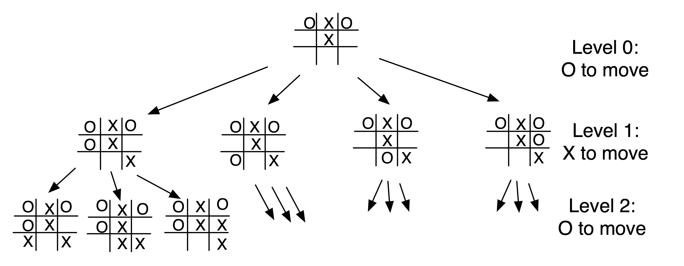
To make the search more efficient, we maintain values for alpha and beta for each search level. Alpha and beta determine the best possible/worst possible move available at a given level. If we reach a situation like the second position in level 2 where X has won, then we can immediately determine that O’s last move in level 1 that produced this position (of allowing X an instant win) is a low valued move for O (but a high valued move for X). This allows us to immediately “prune” the search tree by ignoring all other possible positions arising from the first O move in level 1. This alpha-beta cutoff (or tree pruning) procedure can save a large percentage of search time, especially if we can set the search order at each level with “probably best” moves considered first.
While tree diagrams as seen in the figure showing possible moves for tic-tac-toe quickly get complicated, it is easy for a computer program to generate possible moves, calculate new possible board positions and temporarily store them, and recursively apply the same procedure to the next search level (but switching min-max “sides” in the board evaluation). We will see in the next section that it only requires about 100 lines of Java code to implement an abstract class framework for handling the details of performing an alpha-beta enhanced search. The additional game specific classes for tic-tac-toe require about an additional 150 lines of code to implement; chess requires an additional 450 lines of code.
A Java Framework for Search and Game Playing
The general interface for the Java classes that we will develop in this section was inspired by the Common LISP game-playing framework written by Kevin Knight and described in (Rich, Knight 1991). The abstract class GameSearch contains the code for running a two-player game and performing an alpha-beta search. This class needs to be sub-classed to provide the eight methods:
      public abstract boolean drawnPosition(Position p)
      public abstract boolean wonPosition(Position p,
                                          boolean player)
                      positionEvaluation(Position p,
                                         boolean player)
      public abstract void printPosition(Position p)
      public abstract Position []
                      possibleMoves(Position p,
                                    boolean player)
      public abstract Position makeMove(Position p,
                                        boolean player,
                                        Move move)
      public abstract boolean reachedMaxDepth(Position p,
                                              int depth)
      public abstract Move getMove()
The method drawnPosition should return a Boolean true value if the given position evaluates to a draw situation. The method wonPosition should return a true value if the input position is won for the indicated player. By convention, I use a Boolean true value to represent the computer and a Boolean false value to represent the human opponent. The method positionEvaluation returns a position evaluation for a specified board position and player. Note that if we call positionEvaluation switching the player for the same board position, then the value returned is the negative of the value calculated for the opposing player. The method possibleMoves returns an array of objects belonging to the class Position. In an actual game like chess, the position objects will actually belong to a chess-specific refinement of the Position class (e.g., for the chess program developed later in this chapter, the method possibleMoves will return an array of ChessPosition objects). The method makeMove will return a new position object for a specified board position, side to move, and move. The method reachedMaxDepth returns a Boolean true value if the search process has reached a satisfactory depth. For the tic-tac-toe program, the method reachedMaxDepth does not return true unless either side has won the game or the board is full; for the chess program, the method reachedMaxDepth returns true if the search has reached a depth of 4 half moves deep (this is not the best strategy, but it has the advantage of making the example program short and easy to understand). The method getMove returns an object of a class derived from the class Move (e.g., TicTacToeMove or ChessMove).
The GameSearch class implements the following methods to perform game search:
      protected Vector alphaBeta(int depth, Position p,
                                 boolean player)
      protected Vector alphaBetaHelper(int depth,
                                       Position p,
                                       boolean player,
                                       float alpha,
                                       float beta)
      public void playGame(Position startingPosition,
                           boolean humanPlayFirst)
The method alphaBeta is simple; it calls the helper method alphaBetaHelper with initial search conditions; the method alphaBetaHelper then calls itself recursively. The code for alphaBeta is:
      protected Vector alphaBeta(int depth,
                                 Position p,
                                 boolean player)  {
        Vector v = alphaBetaHelper(depth, p, player,
                                   1000000.0f,
                                  -1000000.0f);
        return v;
      }
It is important to understand what is in the vector returned by the methods alphaBeta and alphaBetaHelper. The first element is a floating point position evaluation for the point of view of the player whose turn it is to move; the remaining values are the “best move” for each side to the last search depth. As an example, if I let the tic-tac-toe program play first, it places a marker at square index 0, then I place my marker in the center of the board an index 4. At this point, to calculate the next computer move, alphaBeta is called and returns the following elements in a vector:
     next element: 0.0
     next element: [-1,0,0,0,1,0,0,0,0,]
     next element: [-1,1,0,0,1,0,0,0,0,]
     next element: [-1,1,0,0,1,0,0,-1,0,]
     next element: [-1,1,0,1,1,0,0,-1,0,]
     next element: [-1,1,0,1,1,-1,0,-1,0,]
     next element: [-1,1,1,1,1,-1,0,-1,0,]
     next element: [-1,1,1,1,1,-1,-1,-1,0,]
     next element: [-1,1,1,1,1,-1,-1,-1,1,]
Here, the alpha-beta enhanced min-max search looked all the way to the end of the game and these board positions represent what the search procedure calculated as the best moves for each side. Note that the class TicTacToePosition (derived from the abstract class Position) has a toString method to print the board values to a string.
The same printout of the returned vector from alphaBeta for the chess program is:
    next element: 5.4
     next element:
         [4,2,3,5,9,3,2,4,7,7,1,1,1,0,1,1,1,1,7,7,
          0,0,0,0,0,0,0,0,7,7,0,0,0,1,0,0,0,0,7,7,
          0,0,0,0,0,0,0,0,7,7,0,0,0,0,-1,0,0,0,7,7,
          -1,-1,-1,-1,0,-1,-1,-1,7,7,-4,-2,-3,-5,-9,
          -3,-2,-4,]
     next element:
         [4,2,3,0,9,3,2,4,7,7,1,1,1,5,1,1,1,1,7,7,
          0,0,0,0,0,0,0,0,7,7,0,0,0,1,0,0,0,0,7,7,
          0,0,0,0,0,0,0,0,7,7,0,0,0,0,-1,0,0,0,7,7,
          -1,-1,-1,-1,0,-1,-1,-1,7,7,-4,-2,-3,-5,-9,
          -3,-2,-4,]
     next element:
         [4,2,3,0,9,3,2,4,7,7,1,1,1,5,1,1,1,1,7,7,
          0,0,0,0,0,0,0,0,7,7,0,0,0,1,0,0,0,0,7,7,
          0,0,0,0,0,0,0,0,7,7,0,0,0,0,-1,-5,0,0,7,7,
          -1,-1,-1,-1,0,-1,-1,-1,7,7,-4,-2,-3,0,-9,
          -3,-2,-4,]
     next element:
         [4,2,3,0,9,3,0,4,7,7,1,1,1,5,1,1,1,1,7,7,
          0,0,0,0,0,2,0,0,7,7,0,0,0,1,0,0,0,0,7,7,
          0,0,0,,0,0,0,0,0,7,7,0,0,0,0,-1,-5,0,0,7,7,
          -1,-1,-1,-1,0,-1,-1,-1,7,7,-4,-2,-3,0,-9,
          -3,-2,-4,]
     next element:
         [4,2,3,0,9,3,0,4,7,7,1,1,1,5,1,1,1,1,7,7,
          0,0,0,0,0,2,0,0,7,7,0,0,0,1,0,0,0,0,7,7,
          -1,0,0,0,0,0,0,0,7,7,0,0,0,0,-1,-5,0,0,7,7,
          0,-1,-1,-1,0,-1,-1,-1,7,7,-4,-2,-3,0,-9,
          -3,-2,-4,]
Here, the search procedure assigned the side to move (the computer) a position evaluation score of 5.4; this is an artifact of searching to a fixed depth. Notice that the board representation is different for chess, but because the GameSearch class manipulates objects derived from the classes Position and Move, the GameSearch class does not need to have any knowledge of the rules for a specific game. We will discuss the format of the chess position class ChessPosition in more detail when we develop the chess program.
The classes Move and Position contain no data and methods at all. The classes Move and Position are used as placeholders for derived classes for specific games. The search methods in the abstract GameSearch class manipulate objects derived from the classes Move and Position.
Now that we have seen the debug printout of the contents of the vector returned from the methods alphaBeta and alphaBetaHelper, it will be easier to understand how the method alphaBetaHelper works. The following text shows code fragments from the alphaBetaHelper method interspersed with book text:
      protected Vector alphaBetaHelper(int depth,
                                       Position p,
                                       boolean player,
                                       float alpha,
                                       float beta) {
Here, we notice that the method signature is the same as for alphaBeta, except that we pass floating point alpha and beta values. The important point in understanding min-max search is that most of the evaluation work is done while “backing up” the search tree; that is, the search proceeds to a leaf node (a node is a leaf if the method reachedMaxDepth return a Boolean true value), and then a return vector for the leaf node is created by making a new vector and setting its first element to the position evaluation of the position at the leaf node and setting the second element of the return vector to the board position at the leaf node:
        if (reachedMaxDepth(p, depth)) {
          Vector v = new Vector(2);
          float value = positionEvaluation(p, player);
          v.addElement(new Float(value));
          v.addElement(p);
          return v;
        }
If we have not reached the maximum search depth (i.e., we are not yet at a leaf node in the search tree), then we enumerate all possible moves from the current position using the method possibleMoves and recursively call alphaBetaHelper for each new generated board position. In terms of the figure showing possible moves for tic-tac-toe, at this point we are moving down to another search level (e.g., from level 1 to level 2; the level in the figure showing possible moves for tic-tac-toe corresponds to depth argument in alphaBetaHelper):
      Vector best = new Vector();
      Position [] moves = possibleMoves(p, player);
      for (int i=0; i<moves.length; i++) {
        Vector v2 = alphaBetaHelper(depth + 1, moves[i],
                                    !player,
                                    -beta, -alpha);
        float value = -((Float)v2.elementAt(0)).floatValue();
        if (value > beta) {
          if(GameSearch.DEBUG)
            System.out.println(" ! ! ! value="+
                               value+
                               ",beta="+beta);
          beta = value;
          best = new Vector();
          best.addElement(moves[i]);
          Enumeration enum = v2.elements();
          enum.nextElement(); // skip previous value
          while (enum.hasMoreElements()) {
            Object o = enum.nextElement();
            if (o != null) best.addElement(o);
          }
        }
        /**
         * Use the alpha-beta cutoff test to abort
         * search if we found a move that proves that
         * the previous move in the move chain was dubious
         */
        if (beta >= alpha) {
          break;
        }
      }
Notice that when we recursively call alphaBetaHelper, we are “flipping” the player argument to the opposite Boolean value. After calculating the best move at this depth (or level), we add it to the end of the return vector:
        Vector v3 = new Vector();
        v3.addElement(new Float(beta));
        Enumeration enum = best.elements();
        while (enum.hasMoreElements()) {
          v3.addElement(enum.nextElement());
        }
        return v3;
When the recursive calls back up and the first call to alphaBetaHelper returns a vector to the method alphaBeta, all of the “best” moves for each side are stored in the return vector, along with the evaluation of the board position for the side to move.
The class GameSearch method playGame is fairly simple; the following code fragment is a partial listing of playGame showing how to call alphaBeta, getMove, and makeMove:
      public void playGame(Position startingPosition,
                           boolean humanPlayFirst) {
        System.out.println("Your move:");
        Move move = getMove();
        startingPosition = makeMove(startingPosition,
                                    HUMAN, move);
        printPosition(startingPosition);
        Vector v = alphaBeta(0, startingPosition, PROGRAM);
        startingPosition = (Position)v.elementAt(1);
        }
      }
The debug printout of the vector returned from the method alphaBeta seen earlier in this section was printed using the following code immediately after the call to the method alphaBeta:
          Enumeration enum = v.elements();
          while (enum.hasMoreElements()) {
            System.out.println(" next element: " +
                               enum.nextElement());
          }
In the next few sections, we will implement a tic-tac-toe program and a chess-playing program using this Java class framework.
Tic-Tac-Toe Using the Alpha-Beta Search Algorithm
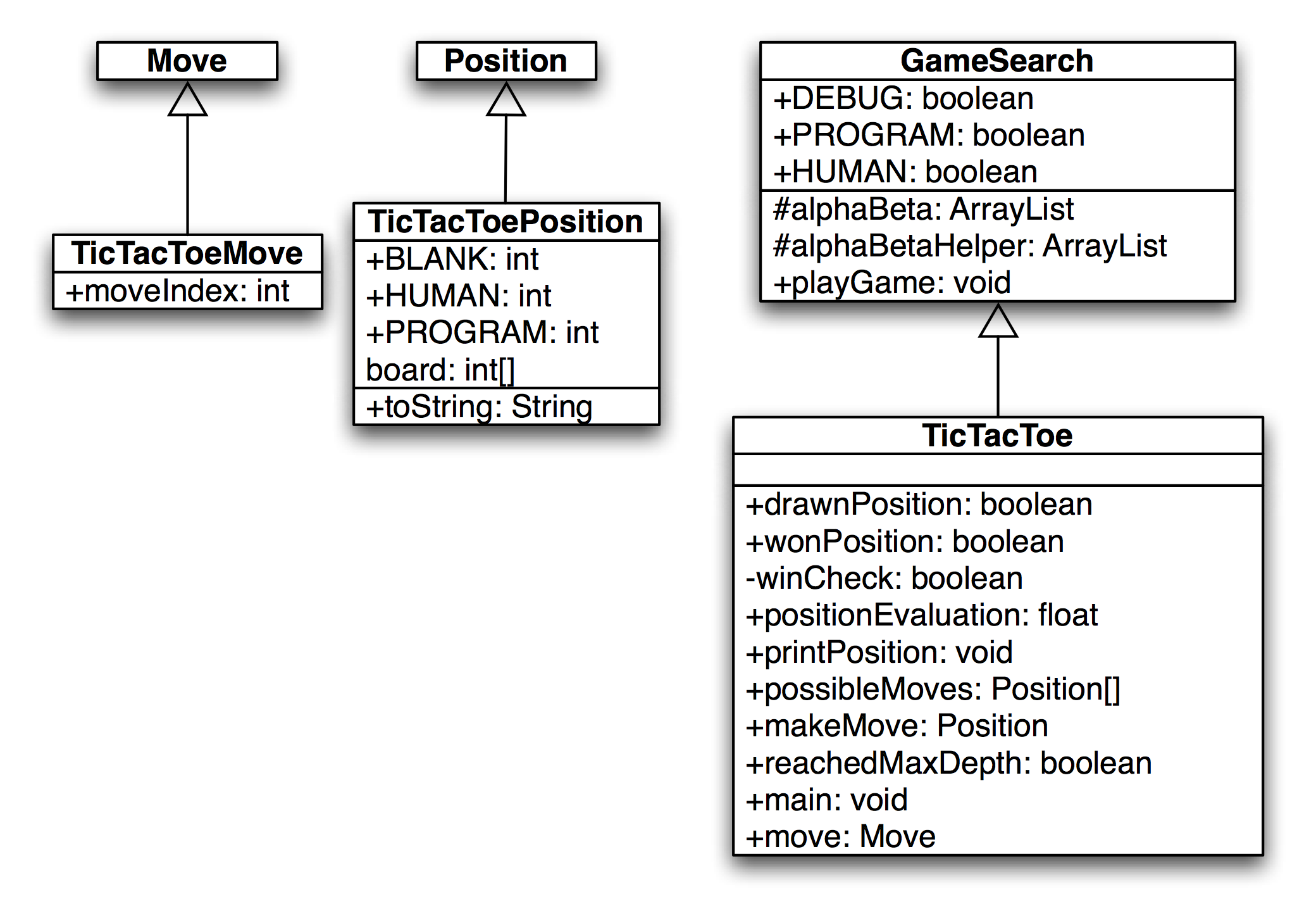
Using the Java class framework of GameSearch, Position, and Move, it is simple to write a basic tic-tac-toe program by writing three new derived classes (as seen in the next figure showing a UML Class Diagram) TicTacToe (derived from GameSearch), TicTacToeMove (derived from Move), and TicTacToePosition (derived from Position).
I assume that the reader has the book example code installed and available for viewing. In this section, I will only discuss the most interesting details of the tic-tac-toe class refinements; I assume that the reader can look at the source code. We will start by looking at the refinements for the position and move classes. The TicTacToeMove class is trivial, adding a single integer value to record the square index for the new move:
    public class TicTacToeMove extends Move {
      public int moveIndex;
    }
The board position indices are in the range of [0..8] and can be considered to be in the following order:
       0 1 2
       3 4 5
       6 7 8
The class TicTacToePosition is also simple:
    public class TicTacToePosition extends Position {
        final static public int BLANK = 0;
        final static public int HUMAN = 1;
        final static public int PROGRAM = -1;
        int [] board = new int[9];
        public String toString() {
            StringBuffer sb = new StringBuffer("[");
            for (int i=0; i<9; i++)
              sb.append(""+board[i]+",");
            sb.append("]");
            return sb.toString();
        }
    }
This class allocates an array of nine integers to represent the board, defines constant values for blank, human, and computer squares, and defines a toString method to print out the board representation to a string.
The TicTacToe class must define the following abstract methods from the base class GameSearch:
     public abstract boolean drawnPosition(Position p)
     public abstract boolean wonPosition(Position p,
                                         boolean player)
     public abstract float positionEvaluation(Position p,
                                              boolean player)
     public abstract void printPosition(Position p)
     public abstract Position [] possibleMoves(Position p,
                                               boolean player)
     public abstract Position makeMove(Position p,
                                       boolean player,
                                       Move move)
     public abstract boolean reachedMaxDepth(Position p,
                                            int depth)
     public abstract Move getMove()
The implementation of these methods uses the refined classes TicTacToeMove and TicTacToePosition. For example, consider the method drawnPosition that is responsible for selecting a drawn (or tied) position:
      public boolean drawnPosition(Position p) {
        boolean ret = true;
        TicTacToePosition pos = (TicTacToePosition)p;
        for (int i=0; i<9; i++) {
          if (pos.board[i] == TicTacToePosition.BLANK){
            ret = false;
            break;
          }
        }
        return ret;
      }
The overridden methods from the GameSearch base class must always cast arguments of type Position and Move to TicTacToePosition and TicTacToeMove. Note that in the method drawnPosition, the argument of class Position is cast to the class TicTacToePosition. A position is considered to be a draw if all of the squares are full. We will see that checks for a won position are always made before checks for a drawn position, so that the method drawnPosition does not need to make a redundant check for a won position. The method wonPosition is also simple; it uses a private helper method winCheck to test for all possible winning patterns in tic-tac-toe. The method positionEvaluation uses the following board features to assign a fitness value from the point of view of either player:
- The number of blank squares on the board
- If the position is won by either side
- If the center square is taken
The method positionEvaluation is simple, and is a good place for the interested reader to start modifying both the tic-tac-toe and chess programs:
        public float positionEvaluation(Position p,
                                        boolean player) {
            int count = 0;
            TicTacToePosition pos = (TicTacToePosition)p;
            for (int i=0; i<9; i++) {
                if (pos.board[i] == 0) count++;
            }
            count = 10 - count;
            // prefer the center square:
            float base = 1.0f;
            if (pos.board[4] == TicTacToePosition.HUMAN &&
                player) {
                base += 0.4f;
            }
            if (pos.board[4] == TicTacToePosition.PROGRAM &&
                !player) {
                base -= 0.4f;
            }
            float ret = (base - 1.0f);
            if (wonPosition(p, player))  {
                return base + (1.0f / count);
            }
            if (wonPosition(p, !player))  {
                return -(base + (1.0f / count));
            }
            return ret;
        }
The only other method that we will look at here is possibleMoves; the interested reader can look at the implementation of the other (very simple) methods in the source code. The method possibleMoves is called with a current position, and the side to move (i.e., program or human):
        public Position [] possibleMoves(Position p,
                                         boolean player) {
            TicTacToePosition pos = (TicTacToePosition)p;
            int count = 0;
            for (int i=0; i<9; i++) {
                if (pos.board[i] == 0) count++;
            }
            if (count == 0) return null;
            Position [] ret = new Position[count];
            count = 0;
            for (int i=0; i<9; i++) {
                if (pos.board[i] == 0) {
                    TicTacToePosition pos2 =
                               new  TicTacToePosition();
                    for (int j=0; j<9; j++)
                         pos2.board[j] = pos.board[j];
                    if (player) pos2.board[i] = 1;
                    else pos2.board[i] = -1;
                    ret[count++] = pos2;
                }
            }
            return ret;
        }
It is very simple to generate possible moves: every blank square is a legal move. (This method will not be as straightforward in the example chess program!)
It is simple to compile and run the example tic-tac-toe program: change directory to src-search-game and type:
    mvn install
    mvn exec:java -Dexec.mainClass="search.game.TicTacToe"
When asked to enter moves, enter an integer between 0 and 8 for a square that is currently blank (i.e., has a zero value). The following shows this labeling of squares on the tic-tac-toe board:
You might need to enter two return (enter) keys after entering your move square when using a macOS terminal.
Chess Using the Alpha-Beta Search Algorithm
Using the Java class framework of GameSearch, Position, and Move, it is reasonably easy to write a simple chess program by writing three new derived classes (see the figure showing a UML diagram for the chess game casses) Chess (derived from GameSearch), ChessMove (derived from Move), and ChessPosition (derived from Position). The chess program developed in this section is intended to be an easy to understand example of using alpha-beta min-max search; as such, it ignores several details that a fully implemented chess program would implement:
- Allow the computer to play either side (computer always plays black in this example).
- Allow en-passant pawn captures.
- Allow the player to take back a move after making a mistake.
The reader is assumed to have read the last section on implementing the tic-tac-toe game; details of refining the GameSearch, Move, and Position classes are not repeated in this section.
The following figure showing a UML diagram for the chess game casses shows the UML class diagram for both the general purpose GameSearch framework and the classes derived to implement chess specific data and behavior.
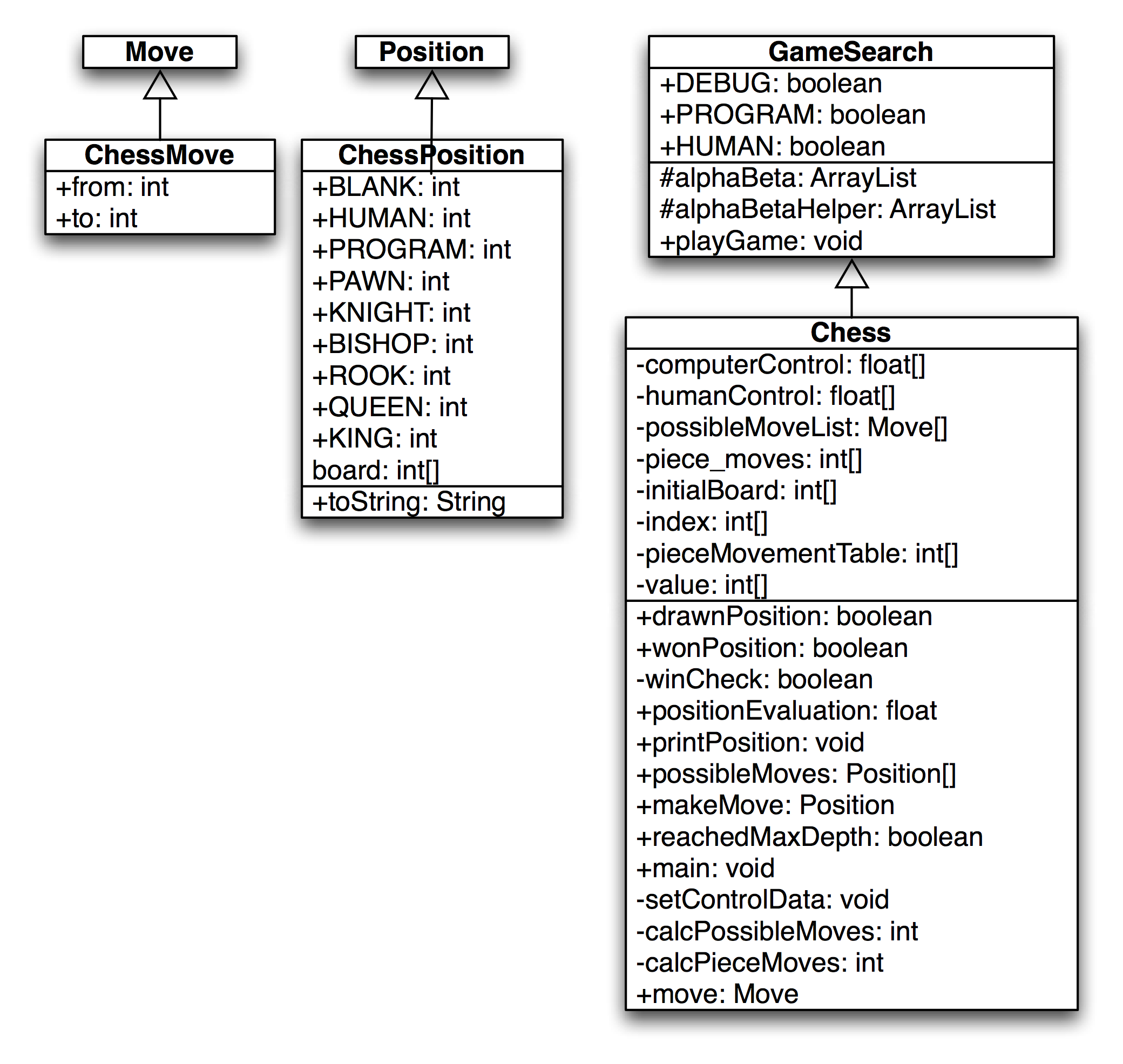
The class ChessMove contains data for recording from and to square indices:
    public class ChessMove extends Move {
        public int from;
        public int to;
    }
The board is represented as an integer array with 120 elements. A chessboard only has 64 squares; the remaining board values are set to a special value of 7, which indicates an “off board” square. The initial board setup is defined statically in the Chess class and the off-board squares have a value of “7”:
    private static int [] initialBoard = {
     7, 7, 7, 7, 7, 7, 7, 7, 7, 7, 7,
     7, 7, 7, 7, 7, 7, 7, 7, 7, 7, 7,
     4, 2, 3, 5, 9, 3, 2, 4, 7, 7,   // white pieces
     1, 1, 1, 1, 1, 1, 1, 1, 7, 7,   // white pawns
     0, 0, 0, 0, 0, 0, 0, 0, 7, 7,   // 8 blank squares
     0, 0, 0, 0, 0, 0, 0, 0, 7, 7,   // 8 blank squares
     0, 0, 0, 0, 0, 0, 0, 0, 7, 7,   // 8 blank squares
     0, 0, 0, 0, 0, 0, 0, 0, 7, 7,   // 8 blank squares
     -1,-1,-1,-1,-1,-1,-1,-1, 7, 7,  // black pawns
     -4,-2,-3,-5,-9,-3,-2,-4, 7, 7,  // black pieces
     7, 7, 7, 7, 7, 7, 7, 7, 7, 7, 7,
     7, 7, 7, 7, 7, 7, 7, 7, 7, 7, 7
    };
It is difficult to see from this listing of the board square values but in effect a regular chess board if padded on all sides with two rows and columns of ``7” values.
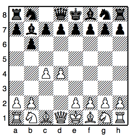
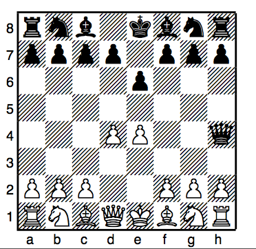
We see the start of a sample chess game in the previous figure and the continuation of this same game in the next figure.The lookahead is limited to 2 moves (4 ply).

The class ChessPosition contains data for this representation and defines constant values for playing sides and piece types:
      public class ChessPosition extends Position {
        final static public int BLANK = 0;
        final static public int HUMAN = 1;
        final static public int PROGRAM = -1;
        final static public int PAWN = 1;
        final static public int KNIGHT = 2;
        final static public int BISHOP = 3;
        final static public int ROOK = 4;
        final static public int QUEEN = 5;
        final static public int KING = 6;
        int [] board = new int[120];
        public String toString() {
            StringBuffer sb = new StringBuffer("[");
            for (int i=22; i<100; i++) {
                sb.append(""+board[i]+",");
            }
            sb.append("]");
            return sb.toString();
        }
      }
The class Chess also defines other static data. The following array is used to encode the values assigned to each piece type (e.g., pawns are worth one point, knights and bishops are worth 3 points, etc.):
      private static int [] value = {
        0, 1, 3, 3, 5, 9, 0, 0, 0, 12
      };
The following array is used to codify the possible incremental moves for pieces:
      private static int [] pieceMovementTable = {
        0, -1, 1, 10, -10, 0, -1, 1, 10, -10, -9, -11, 9,
        11, 0, 8, -8, 12, -12, 19, -19, 21, -21, 0, 10, 20,
        0, 0, 0, 0, 0, 0, 0, 0
      };
The starting index into the pieceMovementTable array is calculated by indexing the following array with the piece type index (e.g., pawns are piece type 1, knights are piece type 2, bishops are piece type 3, rooks are piece type 4, etc.:
      private static int [] index = {
        0, 12, 15, 10, 1, 6, 0, 0, 0, 6
      };
When we implement the method possibleMoves for the class Chess, we will see that except for pawn moves, all other possible piece type moves are very easy to calculate using this static data. The method possibleMoves is simple because it uses a private helper method calcPieceMoves to do the real work. The method possibleMoves calculates all possible moves for a given board position and side to move by calling calcPieceMove for each square index that references a piece for the side to move.
We need to perform similar actions for calculating possible moves and squares that are controlled by each side. In the first version of the class Chess that I wrote, I used a single method for calculating both possible move squares and controlled squares. However, the code was difficult to read, so I split this initial move generating method out into three methods:
- possibleMoves – required because this was an abstract method in GameSearch. This method calls calcPieceMoves for all squares containing pieces for the side to move, and collects all possible moves.
- calcPieceMoves – responsible to calculating pawn moves and other piece type moves for a specified square index.
- setControlData – sets the global array computerControl and humanControl. This method is similar to a combination of possibleMoves and calcPieceMoves, but takes into effect “moves” onto squares that belong to the same side for calculating the effect of one piece guarding another. This control data is used in the board position evaluation method positionEvaluation.
We will discuss calcPieceMoves here, and leave it as an exercise to carefully read the similar method setControlData in the source code. This method places the calculated piece movement data in static storage (the array piece_moves) to avoid creating a new Java object whenever this method is called; method calcPieceMoves returns an integer count of the number of items placed in the static array piece_moves. The method calcPieceMoves is called with a position and a square index; first, the piece type and side are determined for the square index:
      private int calcPieceMoves(ChessPosition pos,
                                 int square_index) {
        int [] b = pos.board;
        int piece = b[square_index];
        int piece_type = piece;
        if (piece_type < 0) piece_type = -piece_type;
        int piece_index = index[piece_type];
        int move_index = pieceMovementTable[piece_index];
        if (piece < 0) side_index = -1;
        else              side_index = 1;
Then, a switch statement controls move generation for each type of chess piece (movement generation code is not shown – see the file Chess.java):
        switch (piece_type) {
        case ChessPosition.PAWN:
          break;
        case ChessPosition.KNIGHT:
        case ChessPosition.BISHOP:
        case ChessPosition.ROOK:
        case ChessPosition.KING:
        case ChessPosition.QUEEN:
          break;
        }
The logic for pawn moves is a little complex but the implementation is simple. We start by checking for pawn captures of pieces of the opposite color. Then check for initial pawn moves of two squares forward, and finally, normal pawn moves of one square forward. Generated possible moves are placed in the static array piece_moves and a possible move count is incremented. The move logic for knights, bishops, rooks, queens, and kings is very simple since it is all table driven. First, we use the piece type as an index into the static array index; this value is then used as an index into the static array pieceMovementTable. There are two loops: an outer loop fetches the next piece movement delta from the pieceMovementTable array and the inner loop applies the piece movement delta set in the outer loop until the new square index is off the board or “runs into” a piece on the same side. Note that for kings and knights, the inner loop is only executed one time per iteration through the outer loop:
        move_index = piece;
        if (move_index < 0) move_index = -move_index;
        move_index = index[move_index];
        //System.out.println("move_index="+move_index);
        next_square =
            square_index + pieceMovementTable[move_index];
      outer:
        while (true) {
          inner:
            while (true) {
              if (next_square > 99) break inner;
              if (next_square < 22) break inner;
              if (b[next_square] == 7) break inner;

              // check for piece on the same side:
              if (side_index < 0 && b[next_square] < 0)
                 break inner;
              if (side_index >0 && b[next_square]  > 0)
                 break inner;

              piece_moves[count++] = next_square;
              if (b[next_square] != 0) break inner;
              if (piece_type == ChessPosition.KNIGHT)
                 break inner;
              if (piece_type == ChessPosition.KING)
                 break inner;
              next_square += pieceMovementTable[move_index];
           }
           move_index += 1;
           if (pieceMovementTable[move_index] == 0)
              break outer;
           next_square = square_index +
                            pieceMovementTable[move_index];
       }
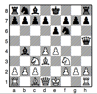
The figures show the start of a second example game. The computer was making too many trivial mistakes in the first game so here I increased the lookahead to 2 1/2 moves. Now the computer takes one to two seconds per move and plays a better game. Increasing the lookahead to 3 full moves yields a better game but then the program can take up to about ten seconds per move.
The method setControlData is very similar to this method; I leave it as an exercise to the reader to read through the source code. Method setControlData differs in also considering moves that protect pieces of the same color; calculated square control data is stored in the static arrays computerControl and humanControl. This square control data is used in the method positionEvaluation that assigns a numerical rating to a specified chessboard position on either the computer or human side. The following aspects of a chessboard position are used for the evaluation:
- material count (pawns count 1 point, knights and bishops 3 points, etc.)
- count of which squares are controlled by each side
- extra credit for control of the center of the board
- credit for attacked enemy pieces
Notice that the evaluation is calculated initially assuming the computer’s side to move. If the position if evaluated from the human player’s perspective, the evaluation value is multiplied by minus one. The implementation of positionEvaluation is:
      public float positionEvaluation(Position p,
                                      boolean player) {
        ChessPosition pos = (ChessPosition)p;
        int [] b = pos.board;
        float ret = 0.0f;
        // adjust for material:
        for (int i=22; i<100; i++) {
          if (b[i] != 0 && b[i] != 7)  ret += b[i];
        }

        // adjust for positional advantages:
        setControlData(pos);
        int control = 0;
        for (int i=22; i<100; i++) {
          control += humanControl[i];
          control -= computerControl[i];
        }
        // Count center squares extra:
        control += humanControl[55] - computerControl[55];
        control += humanControl[56] - computerControl[56];
        control += humanControl[65] - computerControl[65];
        control += humanControl[66] - computerControl[66];

        control /= 10.0f;
        ret += control;

        // credit for attacked pieces:
        for (int i=22; i<100; i++) {
          if (b[i] == 0 || b[i] == 7) continue;
          if (b[i] < 0) {
            if (humanControl[i] > computerControl[i]) {
                ret += 0.9f * value[-b[i]];
            }
          }
          if (b[i] > 0) {
            if (humanControl[i] < computerControl[i]) {
              ret -= 0.9f * value[b[i]];
            }
          }
        }
        // adjust if computer side to move:
        if (!player) ret = -ret;
        return ret;
      }
It is simple to compile and run the example chess program by typing in the search directory:
When asked to enter moves, enter string like “d2d4” to enter a move in chess algebraic notation. Here is sample output from the program:
Note that the newest code in the GitHub repository uses Unicode characters to display graphics for Chess pieces.
The example chess program plays in general good moves, but its play could be greatly enhanced with an “opening book” of common chess opening move sequences. If you run the example chess program, depending on the speed of your computer and your Java runtime system, the program takes a while to move (about 5 seconds per move on my PC). Where is the time spent in the chess program? The following table shows the total runtime (i.e., time for a method and recursively all called methods) and method-only time for the most time consuming methods. Methods that show zero percent method only time used less than 0.1 percent of the time so they print as zero values.
The interested reader is encouraged to choose a simple two-player game, and using the game search class framework, implement your own game-playing program.
Reasoning
While the topic of reasoning may not be as immediately useful for your work as for example deep learning, reasoning is a broad and sometimes useful topic. You might want to just quickly review this chapter and revisit it when and if you need to use any reasoning system. That said, the introductory discussion of logic and reasoning is good background information to know.
In this chapter we will concentrate on the use of the PowerLoom descriptive logic reasoning system. PowerLoom is available with a Java runtime and Java API - this is what I will use for the examples in this chapter. PowerLoom can also be used with other JVM languages like JRuby and Clojure. PowerLoom is also available in Common Lisp and C++ versions.
The PowerLoom system has not been an active project since 2010. As I update this chapter in July 2020, I still consider PowerLoom to be a useful tool for learning about logic based systems and I have attempted to package PowerLoom in a way that will be easy for you to run interactively and I provide a few simple Java examples in the package com.markwatson.powerloom that demonstrate how to embed PowerLoom in your own Java programs. The complete Java source for PowerLoom is in the directory powerloom/src/main/java/edi/isi/powerloom.
Additionally, we will look at different kinds of reasoning systems (the OWL language) in the chapter on the Semantic Web and use this reasoning in the later chapters Automatically Generating Data for Knowledge Graphs and Knowledge Graph Navigator.
While the material in this chapter will get you started with development using a powerful reasoning system and embedding this reasoning system in Java applications, you may want to dig deeper and I suggest sources for further study at the end of this chapter.
PowerLoom is a newer version of the classic Loom Descriptive Logic reasoning system written at ISI although as I mentioned earlier it has not been developed past 2010. At some point you may want to download the entire PowerLoom distribution to get more examples and access to documentation; the PowerLoom web site.
While we will look at an example of embedding the PowerLoom runtime and a PowerLoom model in a Java example program, I want to make a general comment on PowerLoom development: you will spend most of your time interactively running PowerLoom in an interactive shell that lets you type in concepts, relations, rules, and queries and immediately see the results. If you have ever programmed in Lisp, then this mode of interactive programming will be familiar to you. As seen in the next figure, after interactive development you can deploy in a Java application. This style of development supports entering facts and trying rules and relations interactively and as you get things working you can paste what works into a PowerLoom source file. If you have only worked with compiled languages like Java and C++ this development style may take a while to get used to and appreciate. As seen in the next figure the PowerLoom runtime system, with relations and rules, can be embedded in Java applications that typically clear PowerLoom data memory, assert facts from other live data sources, and then use PowerLoom for inferencing.

Logic
We will look at different types of logic and reasoning systems in this section and then later we will get into PowerLoom specific examples. Logic is the basis for both Knowledge Representation and for reasoning about knowledge. We will encode knowledge using logic and see that we can then infer new facts that are not explicitly asserted. In AI literature you often see discussions of implicit vs. explicit knowledge. Implicit knowledge is inferred from explicitly stated information by using a reasoning system.
First Order Logic was invented by the philosophers Frege and Peirce and is the most widely studied logic system. Unfortunately, full First Order Logic is not computationally tractable for most non-trivial problems so we use more restricted logics. We will use two reasoning systems in this book that support more limited logics:
- We use PowerLoom in this chapter. PowerLoom supports a combination of limited first order predicate logic and features of description logic. PowerLoom is able to classify objects, use rules to infer facts from existing facts and to perform subsumption (determining class membership of instances).
- We will use RDF Schema (RDFS) reasoning in the Chapter on Semantic Web. RDFS supports more limited reasoning than descriptive logic reasoners like PowerLoom and OWL Description Logic reasoners.
History of Logic
The Greek philosopher Aristotle studied forms of logic as part of his desire to improve the representation of knowledge. He started a study of logic and the definition of both terms (e.g., subjects, predicates, nouns, verbs) and types of logical deduction. Much later the philosopher Frege defined predicate logic (for example: All birds have feathers. Brady is a bird, therefore Brady has feathers) that forms the basis for the modern Prolog programming language.
Examples of Different Logic Types
Propositional logic is limited to atomic statements that can be either true or false:
First Order Predicate Logic allows access to the structure of logic statements dealing with predicates that operate on atoms. To use a Prolog notation:
    feathers(X) :- bird(X).
    bird(brady).
In this example, “feathers” and “bird” are predicates and “brady” is an atom. The first example states that for all X, if X is a bird, then X has feathers. In the second example we state that Brady is a bird. Notice that in the Prolog notation that we are using, variables are capitalized and predicate names and literal atoms are lower case.
Here is a query that asks who has feathers:
    ?- feathers(X).
    X = brady
In this example through inference we have determined a new fact, that Brady has feathers because we know that Brady is a bird and we have the rule (or predicate) stating that all birds have feathers. Prolog is not strictly a pure logic programming language since the order in which rules (predicates) are defined changes the inference results. Prolog is a great language for some types of projects (I have used Prolog in both natural language processing and in planning systems). We will see that PowerLoom is considerably more flexible than Prolog but does have a steep learning curve.
Description Logic deals with descriptions of concepts and how these descriptions define the domain of concepts. In terms used in object oriented programming languages: membership in a class is determined implicitly by the description of the object and not by explicitly stating something like “Brady is a member of the bird class.” Description logics divide statements into relations (historically referred to as TBox) and concepts (historically called ABox). We would say that a statement like “All birds have feathers” is stored in the TBox while a specific assertion like “Brady is a bird” is stored in the ABox.
PowerLoom Overview
PowerLoom is designed to be an expressive language for knowledge representation and reasoning. As a result, PowerLoom is not a complete reasoning system but makes tradeoffs for completeness of inferences and expressivity vs. computational efficiency. It is interesting to note that Loom and PowerLoom were designed and implemented to solve real world problems and the tradeoffs to make these problems computationally tractable have informed the design and implementation of these systems. PowerLoom does not make all possible inferences from concepts that it operates on.
The PowerLoom distribution contains two very detailed examples for representing relationships between companies and for information dealing with airplanes. These examples are more detailed than the simpler examples in this chapter. We will look at just one of these examples (business rules and relations) and after working through this chapter, I encourage you to interactively experiment with the two examples that ship with PowerLoom.
We will start by defining some terms used in PowerLoom:
- concept - the Java equivalent would be an instance of a class.
- relation - specifies a link between two concepts.
- function - functional mapping of one concept to another.
- rule - allows new concepts to be deduced without explicitly asserting them.
A relation can specify the types of concepts that a relation connects. An example will make this clear and introduce the Lisp-like syntax of PowerLoom statements:
1     ;;; Concepts:
2     (defconcept person)
3     (defconcept parent (?p person))
4
5     ;;; Relation:
6     (defrelation parent-of ((?p1 parent) (?p2 person)))
Here I have defined two concepts: person and parent. Note that we have a hierarchy of concept types: the parent is a more specific concept type than the person concept. I loose metaphor is that in object oriented programming a parent is a subclass of a person and this hierarchy is stated in line 3 of the last listing. All instances that are parents are also of type person. The relation parent-of links a parent concept to a person concept.
We will learn more about basic PowerLoom functionality in the next two sections as we use PowerLoom in an interactive session and when we embed PowerLoom in a Java example program.
Running PowerLoom Interactively
We will experiment with PowerLoom concepts, relations, and rules in this section in an interactive command shell. I will introduce more examples of PowerLoom functionality for asserting instances of concepts, performing queries, loading PowerLoom source files, defining relations, using separate modules, and asking PowerLoom to explain the inference process that it used for query processing.
You can run PowerLoom using the command line interface using:
cd powerloom
mvn install
mvn exec:java -Dexec.mainClass="edu.isi.powerloom.PowerLoom"
This starts the PowerLoom standalone system and prints a prompt that includes the name of the current module. The default module name is “PL-USER”. In the first example, when I enter the person concept at the interactive prompt then PowerLoom prints the result of the expression that just entered. You can enter (demo) to have access to all of the demo scripts from the PowerLoom distribution. These demo files are in the subdirectory powerloom/sources/logic/demos in the GitHub repository for this book.
Please note that depending on which terminal you are running in, the prompt “PL-USER” does not occur until after entering an “extra” return or enter key.
Now that we have entered two concepts, a test relation, and asserted a few facts, we can look at an example of PowerLoom’s query language:
The obvious point to note from this example is that we never specified that Ken was a parent; rather, PowerLoom deduced this from the parent-of relation. The asserted data is explicit data while the inferred data is implicit and only exists when required to reason over a query.
PowerLoom’s command line system prompts you with the string ``PL-USER |=`` and you can type any definition or query. Like Lisp, PowerLoom uses a prefix notation and expressions are contained in parenthesis. PowerLoom supports a module system for partitioning concepts, relations, functions, and rules into different sets and as previously mentioned “PL-USER” is the default module. PowerLoom modules can form a hierarchy, inheriting concepts, relations, and rules from parent modules.
The subdirectory test_data contains the demo file business.plm written by Robert MacGregor that is supplied with the full PowerLoom distribution. You can load his complete example using:
PL-USER |= (load "test_data/business.plm")
This is a good example because it demonstrates most of the available functionality of PowerLoom in a short 200 lines. When you are finished reading this chapter, please take a few minutes to read through this example file since I do not list all of it it here. There are a few things to notice in this example. Here we see a rule used to make the relation “contains” transitive:
The operator => means that if the first clause is true then so is the second. In English, this rule could be stated “if an instance i1 contains i2 and if instance i2 contains i3 then we can infer that i1 also contains i3.” To see how this rule works in practice, we can switch to the example module “BUSINESS” and find all locations contained inside another location:
Here we have fifteen solutions even though there are only seven contains relations asserted in the business.plm file, the other eight solutions were inferred. In addition to the retrieve function that finds solutions matching a query you can also use the ask function to determine if a specified relation is true; for example:
For complex queries you can use the “why” function to see how PowerLoom solved the last query:
By default the explanation facility is turned off because it causes PowerLoom to run more slowly; it was turned on in the file business.plm using the statement:
Using the PowerLoom APIs in Java Programs
Once you interactively develop concepts, rules and relations then it is likely that you may want to use them with PowerLoom in an embedded mode, making PowerLoom a part of your application. I will get you started with a few Java example programs. The source code for this chapter divide into two packages:
- edu.isi.powerloom - source code from the PowerLoom web site.
- com.markwatson.powerloom - book example code for utilities and two embedded examples.
These packages can be seen in this screen shot:
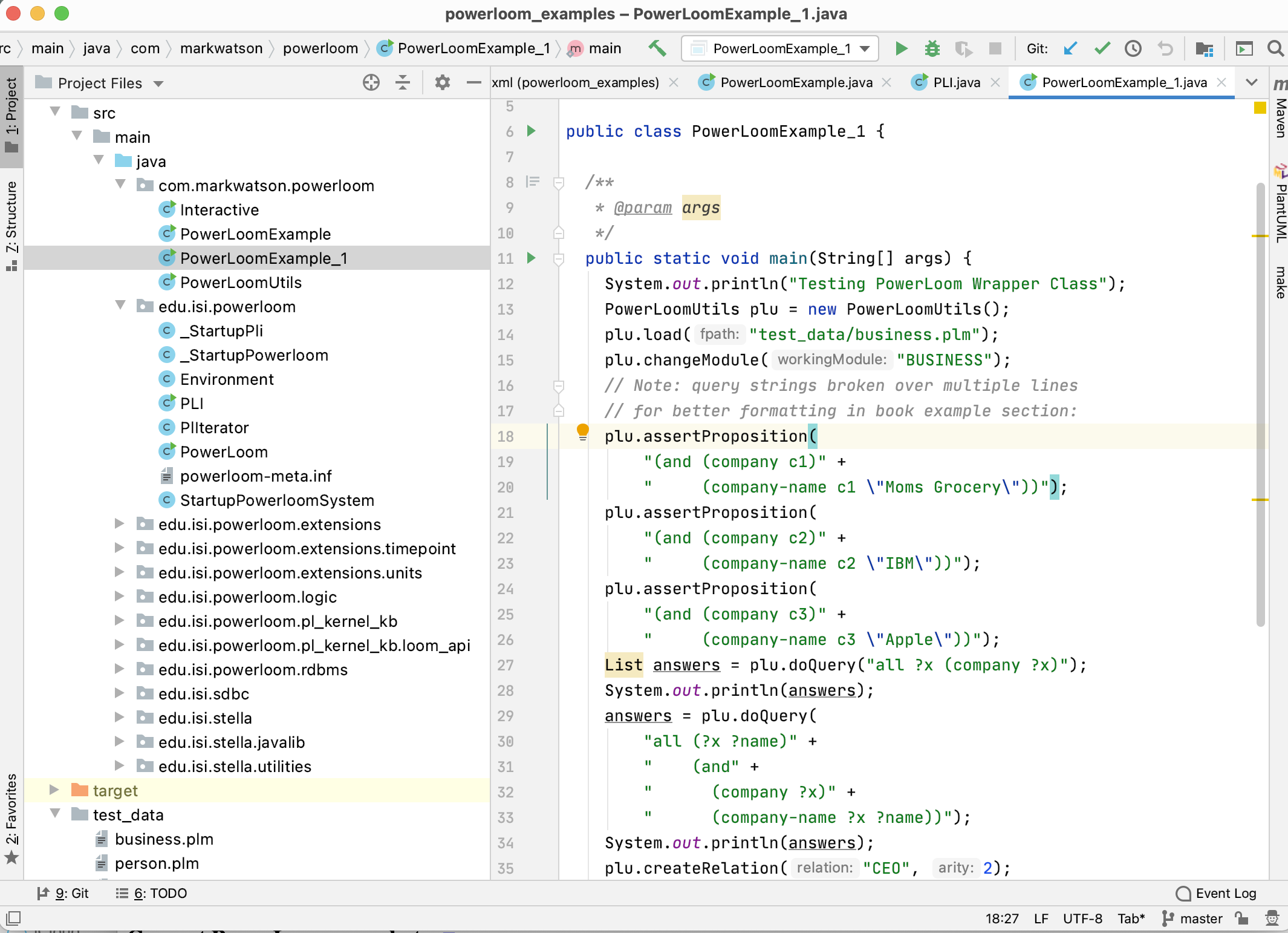
If you download the PowerLoom manual (a PDF file) from the PowerLoom web site, you will have the complete Java API documentation for the Java version of PowerLoom (there are also C++ and Common Lisp versions with separate documentation). I have found that I generally use just a small subset of the Java PowerLoom APIs and I have “wrapped” this subset in a wrapper class in the file PowerLoomUtils.java. We will use my wrapper class for the examples in the rest of this chapter.
The following UML class diagram will give you an overview before we dive into the code:
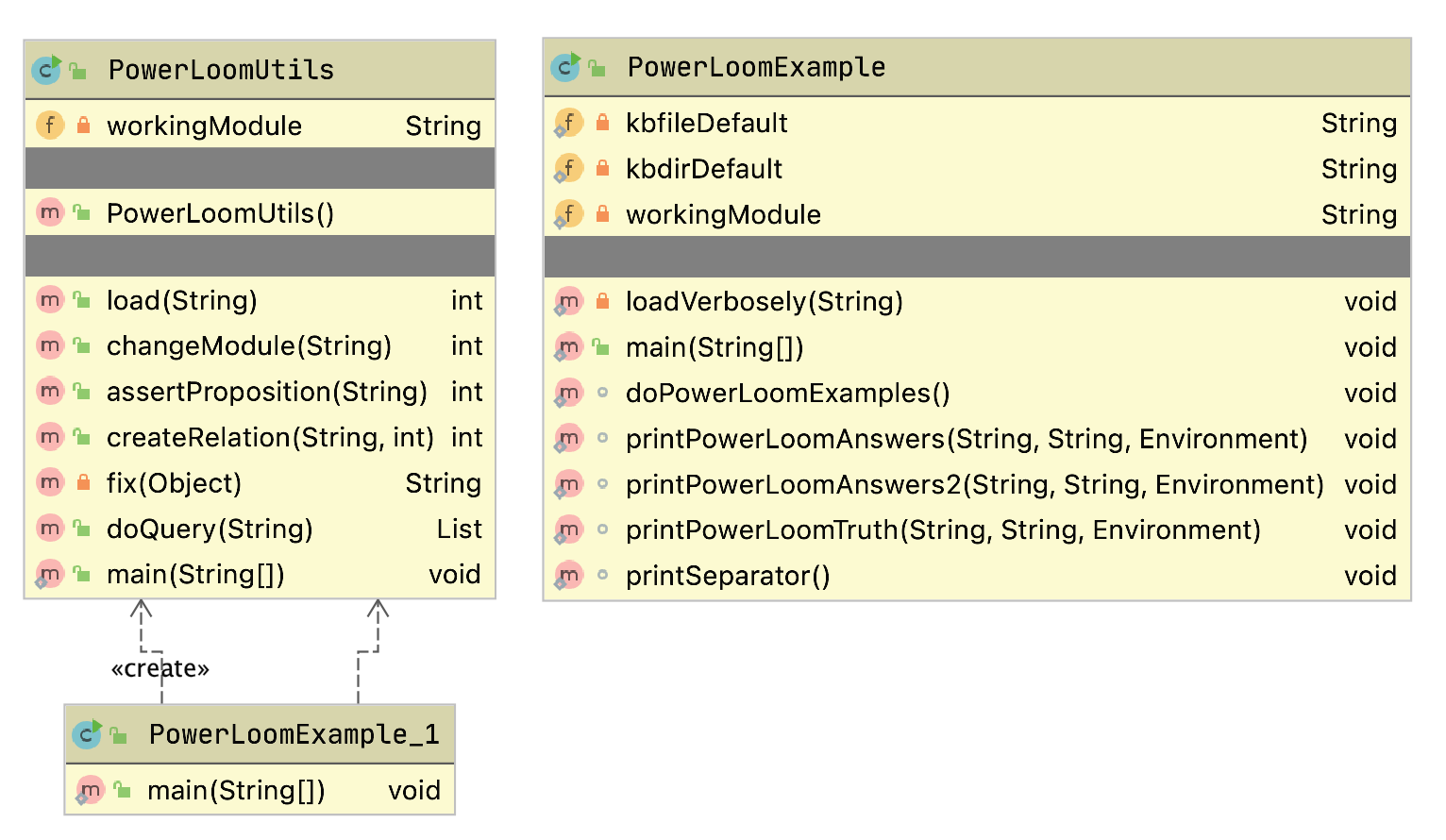
My wrapper class has the follow public methods:
- PowerLoomUtils() - constructor initializes the Java PowerLoom runtime system.
- load(String fpath) - load a source *.plm file.
- changeModule(String workingModule) - set the current PowerLoom working module (“PL-USER” is the default module).
- assertProposition(String proposition) - asserts a new proposition; for example: “(and (company c3) (company-name c3 \“Moms Grocery\”))”. Note that quotation marks are escaped with a backslash character. You can also use single quote characters like: “(and (company c3) (company-name c3 ’Moms Grocery’))” because I convert single quotes in my wrapper code.
- createRelation(String relation, int arity) - create a new relation with a specified arity (number of “arguments”). For example you could create a relation “owns” with arity 2 and then assert “(owns Elaine ’Moms Grocery’)” - I usually do not use this API since I prefer to place relations (with rules) in a source code file ending in the extension *.plm.
- doQuery(String query) - returns a list of results from a query. Each result in the list is itself a list.
You will always want to work in an interactive PowerLoom console for writing and debugging PowerLoom models. I copied the model in business.plm from the PowerLoom distribution to the subdirectory test_data. Here we use it in an embedded Java example in the file PowerLoomExample_1.java:
    PowerLoomUtils plu = new PowerLoomUtils();
    plu.load("test_data/business.plm");
    plu.changeModule("BUSINESS");
    plu.assertProposition(
         "(and (company c1)" +
         "     (company-name c1 \"Moms Grocery\"))");
    plu.assertProposition(
         "(and (company c2)" +
          "     (company-name c2 \"IBM\"))");
    plu.assertProposition(
         "(and (company c3)" +
         "     (company-name c3 \"Apple\"))");
    List answers = plu.doQuery("all ?x (company ?x)");
    System.out.println(answers);
    // answers: [[C3], [C2], [C1]]
    answers = plu.doQuery(
         "all (?x ?name)" +
         "    (and" +
         "      (company ?x)" +
         "      (company-name ?x ?name))");
    System.out.println(answers);
    // answers:
    //   [[C3, "Apple"],
    //    [C2, "IBM"],
    //    [C1, "Moms Grocery"]]
    plu.createRelation("CEO", 2);
    plu.assertProposition(
         "(CEO \"Apple\" \"SteveJobs\")");
    answers = plu.doQuery(
         "all (?x ?name ?ceo)" +
         "    (and" +
         "      (company-name ?x ?name)" +
         "      (CEO ?name ?ceo))");
    System.out.println(answers);
    // answers: [[C3, "Apple", "SteveJobs"]]
I have added the program output produced by printing the value of the list variable “answers” as comments after each System.out.println call. In the wrapper API calls that take a string argument, I broke long strings over several lines for formatting to the width of a page; you would not do this in your own programs because of the cost of the extra string concatenation.
We will not look at the implementation of the PowerLoomUtils class, you can read the code if you are interested. That said, I will make a few comments on the Java PowerLoom APIs. The class PLI contains static methods for initializing the system, loading PowerLoom source files. Here are a few examples:
      PLI.initialize();
      PLI.load("business.plm", null);
      PLI.changeModule("BUSINESS", null);
Suggestions for Further Study
This chapter has provided a brief introduction to PowerLoom. I also showed you how to go about embedding PowerLoom in your Java programs to add capabilities for knowledge representation and reasoning. Assuming that you see benefit to further study I recommend reading through the PowerLoom manual and the presentations (PDF files) on the PowerLoom web site. As you read through this material it is best to have an interactive PowerLoom session open to try the examples as you read them.
Knowledge Representation and Logic are huge subjects and I will close out this chapter by recommending a few books that have been the most helpful to me:
- Knowledge Representation by John Sowa. This has always been my favorite reference for knowledge representation, logic, and ontologies.
- Artificial Intelligence, A Modern Approach by Stuart Russell and Peter Norvig. A very good theoretical treatment of logic and knowledge representation.
- The Art of Prolog by Leon Sterling and Ehud Shapiro. Prolog implements a form of predicate logic that is less expressive than the descriptive logics supported by PowerLoom and OWL (Chapter on Semantic Web). That said, Prolog is very efficient and fairly easy to learn and so is sometimes a better choice. This book is one of my favorite general Prolog references.
The Prolog language is a powerful AI development tool. Both open source, the SWI-Prolog and Amzi Prolog systems have good Java interfaces. I don’t cover Prolog in this book but there are several very good tutorials on the web if you decide to experiment with Prolog.
We will continue in the chapter on the Semantic Web with our study of logic-based reasoning systems in the context of the Semantic Web.
Anomaly Detection Machine Learning Example
Anomaly detection models are used in one very specific class of use cases: when you have many negative (non-anomaly) examples and relatively few positive (anomaly) examples. We can refer to this as an unbalanced training set. For training we will ignore positive examples, create a model of “how things should be,” and hopefully be able to detect anomalies different from the original negative examples.
If you have a large training set of both negative and positive examples then do not use anomaly detection models. If your training examples are balanced then use a classification model as we will see later in the chapter Deep Learning Using Deeplearning4j.
Motivation for Anomaly Detection
There are two other examples in this book using the University of Wisconsin cancer data. These other examples are supervised learning. Anomaly detection as we do it in this chapter is, more or less, unsupervised learning.
When should we use anomaly detection? You should use supervised learning algorithms like neural networks and logistic classification when there are roughly equal number of available negative and positive examples in the training data. The University of Wisconsin cancer data set is fairly evenly split between negative and positive examples.
Anomaly detection should be used when you have many negative (“normal”) examples and relatively few positive (“anomaly”) examples. For the example in this chapter we will simulate scarcity of positive (“anomaly”) results by preparing the data using the Wisconsin cancer data as follows:
- We will split the data into training (60%), cross validation (20%) and testing (20%).
- For the training data, we will discard all but two positive (“anomaly”) examples. We do this to simulate the real world test case where some positive examples are likely to end up in the training data in spite of the fact that we would prefer the training data to only contain negative (“normal”) examples.
- We will use the cross validation data to find a good value for the epsilon meta parameter.
- After we find a good epsilon value, we will calculate the F1 measurement for the model.
Math Primer for Anomaly Detection
We are trying to model “normal” behavior and we do this by taking each feature and fitting a Gaussian (bell curve) distribution to each feature. The learned parameters for a Gaussian distribution are the mean of the data (where the bell shaped curve is centered) and the variance. You might be more familiar with the term standard deviation, \(\sigma\). Variance is defined as \( \sigma ^2\).
We will need to calculate the probability of a value x given the mean and variance of a probability distribution: \(P(x : \mu, \sigma ^2)\) where \(\mu\) is the mean and \( \sigma ^2\) is the squared variance:
$$ P(x : \mu, \sigma ^2) = \frac{1}{{\sigma \sqrt {2\pi } }}e^{{{ - \left( {x - \mu } \right)^2 } \mathord{\left/ {\vphantom {{ - \left( {x - \mu } \right)^2 } {2\sigma ^2 }}} \right. \kern-\nulldelimiterspace} {2\sigma ^2 }}} $$where \(x_i\) are the samples and we can calculate the squared variance as:
$$ \sigma^2 = \frac{\displaystyle\sum_{i=1}^{m}(x_i - \mu)^2} {m} $$We calculate the parameters of \(\mu\) and \( \sigma ^2\) for each feature. A bell shaped distribution in two dimensions is easy to visualize as is an inverted bowl shape in three dimentions. What if we have many features? Well, the math works and don’t worry about not being able to picture it in your mind.
AnomalyDetection Utility Class
The class AnomalyDetection developed in this section is fairly general purpose. It processes a set of training examples and for each feature calculates \(\mu\) and \( \sigma ^2\). We are also training for a third parameter: an epsilon “cutoff” value: if for a given input vector if \(P(x : \mu, \sigma ^2)\) evaluates to a value greater than epsilon then the input vector is “normal”, less than epsilon implies that the input vector is an “anomaly.” The math for calulating these three features from training data is fairly easy but the code is not: we need to organize the training data and search for a value of epsilon that minimizes the error for a cross validaton data set.
To be clear: we separate the input examples into three separate sets of training, cross validation, and testing data. We use the training data to set the model parameters, use the cross validation data to learn an epsilon value, and finally use the testing data to get precision, recall, and F1 scores that indicate how well the model detects anomalies in data not used for training and cross validation.
I present the example program as one long listing, with more code explanation after the listing. Please note the long loop over each input training example starting at line 28 and ending on line 74. The code in lines 25 through 44 processes the input training data sample into three disjoint sets of training, cross validation, and testing data. Then the code in lines 45 through 63 copies these three sets of data to Java arrays.
The code in lines 65 through 73 calculates, for a training example, the value of \(\mu\) (the varible mu in the code).
Please note in the code example that I prepend class variables used in methods with “this.” even when it is not required. I do this for legibility and is a personal style.
The following UML class diagram will give you an overview before we dive into the code:
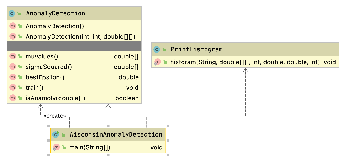
  1 package com.markwatson.anomaly_detection;
  2
  3 import java.util.ArrayList;
  4 import java.util.List;
  5
  6 /**
  7  * Created by markw on 10/7/15.
  8  */
  9 public class AnomalyDetection {
 10
 11   public AnomalyDetection() { }
 12
 13   /**
 14    * AnomalyDetection is a general purpose class for building anomaly detection
 15    * models. You should use this type of mdel when you have mostly negative
 16    * training examples with relatively few positive examples and you need a model
 17    * that detects postive (anomaly) inputs.
 18    *
 19    * @param num_features
 20    * @param num_training_examples
 21    * @param training_examples [num_training_examples][num_features]
 22    */
 23   public AnomalyDetection(int num_features, int num_training_examples,
 24                           double [][] training_examples) {
 25     List<double[]> training = new ArrayList<>();
 26     List<double []> cross_validation = new ArrayList<>();
 27     List<double []> testing = new ArrayList<>();
 28     int outcome_index = num_features - 1; // index of target outcome
 29     for (int i=0; i<num_training_examples; i++) {
 30       if (Math.random() < 0.6) { // 60% training
 31         // Only keep normal (negative) examples in training, except
 32         // remember the reason for using this algorithm is that it
 33         // works with many more negative examples than positive
 34         // examples, and that the algorithm works even with some positive
 35         // examples mixed into the training set. The random test is to
 36         // allow about 10% positive examples to get into the training set:
 37         if (training_examples[i][outcome_index] < 0.5 || Math.random() < 0.1)
 38           training.add(training_examples[i]);
 39       } else if (Math.random() < 0.7) {
 40           cross_validation.add(training_examples[i]);
 41       } else {
 42         testing.add(training_examples[i]);
 43       }
 44     }
 45     this.num_training_examples = training.size();
 46     this.num_cross_validation_examples = cross_validation.size();
 47     this.num_testing_examples = testing.size();
 48
 49     this.training_examples = new double[this.num_training_examples][];
 50     for (int k=0; k<this.num_training_examples; k++) {
 51       this.training_examples[k] = training.get(k);
 52     }
 53
 54     this.cross_validation_examples = new double[num_cross_validation_examples][];
 55     for (int k=0; k<num_cross_validation_examples; k++) {
 56       this.cross_validation_examples[k] = cross_validation.get(k);
 57     }
 58
 59     this.testing_examples = new double[num_testing_examples][];
 60     for (int k=0; k<num_testing_examples; k++) {
 61       // dimensions of [num_training_examples][num_features]:
 62       this.testing_examples[k] = testing.get(k);
 63     }
 64
 65     this.mu = new double[num_features];
 66     this.sigma_squared = new double[num_features];
 67     this.num_features = num_features;
 68     for (int nf = 0; nf < this.num_features; nf++) { //
 69       double sum = 0;
 70       for (int nt = 0; nt < this.num_training_examples; nt++)
 71         sum += training_examples[nt][nf];
 72       this.mu[nf] = sum / this.num_training_examples;
 73     }
 74   }
 75
 76   public double [] muValues()     { return mu; }
 77   public double [] sigmaSquared() { return sigma_squared; }
 78   public double bestEpsilon()     { return best_epsilon; }
 79
 80   /**
 81    *
 82    * Train the model using a range of epsilon values. Epsilon is a
 83    * hyper parameter that we want to find a value that
 84    * minimizes the error count.
 85    */
 86   public void train() {
 87     double best_error_count = 1e10;
 88     for (int epsilon_loop=0; epsilon_loop<40; epsilon_loop++) {
 89       double epsilon = 0.05 + 0.01 * epsilon_loop;
 90       double error_count = train(epsilon);
 91       if (error_count < best_error_count) {
 92         best_error_count = error_count;
 93         best_epsilon = epsilon;
 94       }
 95     }
 96     System.out.println("\n**** Best epsilon value = " + best_epsilon );
 97
 98     // retrain for the best epsilon setting the maximum likelyhood parameters
 99     // which are now in epsilon, mu[] and sigma_squared[]:
100     train_helper(best_epsilon);
101
102     // finally, we are ready to see how the model performs with test data:
103     test(best_epsilon);
104   }
105
106   /**
107    * calculate probability p(x; mu, sigma_squared)
108    *
109    * @param x - example vector
110    * @return
111    */
112   private double p(double [] x) {
113     double sum = 0;
114     // use (num_features - 1) to skip target output:
115     for (int nf=0; nf<num_features - 1; nf++) {
116       sum += (1.0 / (SQRT_2_PI * sigma_squared[nf])) *
117              Math.exp(- (x[nf] - mu[nf]) * (x[nf] - mu[nf]));
118     }
119     return sum / num_features;
120   }
121
122   /**
123    * returns 1 if input vector is an anoomaly
124    *
125    * @param x - example vector
126    * @return
127    */
128   public boolean isAnamoly(double [] x) {
129     double sum = 0;
130     // use (num_features - 1) to skip target output:
131     for (int nf=0; nf<num_features - 1; nf++) {
132       sum += (1.0 / (SQRT_2_PI * sigma_squared[nf])) *
133              Math.exp(- (x[nf] - mu[nf]) * (x[nf] - mu[nf]));
134     }
135     return (sum / num_features) < best_epsilon;
136   }
137
138   private double train_helper_(double epsilon) {
139     // use (num_features - 1) to skip target output:
140     for (int nf = 0; nf < this.num_features - 1; nf++) {
141       double sum = 0;
142       for (int nt=0; nt<this.num_training_examples; nt++) {
143         sum += (this.training_examples[nt][nf] - mu[nf]) *
144                (this.training_examples[nt][nf] - mu[nf]);
145       }
146       sigma_squared[nf] = (1.0 / num_features) * sum;
147     }
148     double cross_validation_error_count = 0;
149     for (int nt=0; nt<this.num_cross_validation_examples; nt++) {
150       double[] x = this.cross_validation_examples[nt];
151       double calculated_value = p(x);
152       if (x[9] > 0.5) { // target training output is ANOMALY
153         // if the calculated value is greater than epsilon
154         // then this x vector is not an anomaly (e.g., it
155         // is a normal sample):
156         if (calculated_value > epsilon) cross_validation_error_count += 1;
157       } else { // target training output is NORMAL
158         if (calculated_value < epsilon) cross_validation_error_count += 1;
159       }
160     }
161     System.out.println("   cross_validation_error_count = " +
162                        cross_validation_error_count +
163                        " for epsilon = " + epsilon);
164     return cross_validation_error_count;
165   }
166
167   private double test(double epsilon) {
168     double num_false_positives = 0, num_false_negatives = 0;
169     double num_true_positives = 0, num_true_negatives = 0;
170     for (int nt=0; nt<this.num_testing_examples; nt++) {
171       double[] x = this.testing_examples[nt];
172       double calculated_value = p(x);
173       if (x[9] > 0.5) { // target training output is ANOMALY
174         if (calculated_value > epsilon) num_false_negatives++;
175         else                            num_true_positives++;
176       } else { // target training output is NORMAL
177         if (calculated_value < epsilon) num_false_positives++;
178         else                            num_true_negatives++;
179       }
180     }
181     double precision = num_true_positives /
182                        (num_true_positives + num_false_positives);
183     double recall = num_true_positives /
184                     (num_true_positives + num_false_negatives);
185     double F1 = 2 * precision * recall / (precision + recall);
186
187     System.out.println("\n\n -- best epsilon = " + this.best_epsilon);
188     System.out.println(" -- number of test examples = " +
189                        this.num_testing_examples);
190     System.out.println(" -- number of false positives = " + num_false_positives);
191     System.out.println(" -- number of true positives = " + num_true_positives);
192     System.out.println(" -- number of false negatives = " + num_false_negatives);
193     System.out.println(" -- number of true negatives = " + num_true_negatives);
194     System.out.println(" -- precision = " + precision);
195     System.out.println(" -- recall = " + recall);
196     System.out.println(" -- F1 = " + F1);
197     return F1;
198   }
199
200   double best_epsilon = 0.02;
201   private double [] mu;  // [num_features]
202   private double [] sigma_squared; // [num_features]
203   private int num_features;
204   private static double SQRT_2_PI = 2.50662827463;
205
206
207   private double[][] training_examples; // [num_features][num_training_examples]
208   // [num_features][num_training_examples]:
209   private double[][] cross_validation_examples;
210   private double[][] testing_examples; // [num_features][num_training_examples]
211   private int num_training_examples;
212   private int num_cross_validation_examples;
213   private int num_testing_examples;
214
215 }
Once the training data and the values of \(\mu\) (the varible mu in the code) are defined for each feature we can define the method train in lines 86 through 104 that calculated the best epsilon “cutoff” value for the training data set using the method train_helper defined in lines 138 through 165. We use the “best” epsilon value by testing with the separate cross validation data set; we do this by calling the method test that is defined in lines 167 through 198.
Example Using the University of Wisconsin Cancer Data
The example in this section loads the University of Wisconsin data and uses the class AnomalyDetection developed in the last section to find anomalies, which for this example will be input vectors that represented malignancy in the original data.
 1 package com.markwatson.anomaly_detection;
 2
 3 import java.io.*;
 4 import org.apache.commons.io.FileUtils;
 5
 6 /**
 7  * Train a deep belief network on the University of Wisconsin Cancer Data Set.
 8  */
 9 public class WisconsinAnomalyDetection {
10
11   private static boolean PRINT_HISTOGRAMS = true;
12
13   public static void main(String[] args) throws Exception {
14
15     String [] lines =
16       FileUtils.readFileToString(
17          new File("data/cleaned_wisconsin_cancer_data.csv")).split("\n");
18     double [][] training_data = new double[lines.length][];
19     int line_count = 0;
20     for (String line : lines) {
21       String [] sarr = line.split(",");
22       double [] xs = new double[10];
23       for (int i=0; i<10; i++) xs[i] = Double.parseDouble(sarr[i]);
24       for (int i=0; i<9; i++) xs[i] *= 0.1;
25       xs[9] = (xs[9] - 2) * 0.5; // make target output be [0,1] instead of [2,4]
26       training_data[line_count++] = xs;
27     }
28
29     if (PRINT_HISTOGRAMS) {
30       PrintHistogram.historam("Clump Thickness", training_data, 0, 0.0, 1.0, 10);
31       PrintHistogram.historam("Uniformity of Cell Size", training_data,
32                               1, 0.0, 1.0, 10);
33       PrintHistogram.historam("Uniformity of Cell Shape", training_data,
34                               2, 0.0, 1.0, 10);
35       PrintHistogram.historam("Marginal Adhesion", training_data,
36                               3, 0.0, 1.0, 10);
37       PrintHistogram.historam("Single Epithelial Cell Size", training_data,
38                               4, 0.0, 1.0, 10);
39       PrintHistogram.historam("Bare Nuclei", training_data, 5, 0.0, 1.0, 10);
40       PrintHistogram.historam("Bland Chromatin", training_data, 6, 0.0, 1.0, 10);
41       PrintHistogram.historam("Normal Nucleoli", training_data, 7, 0.0, 1.0, 10);
42       PrintHistogram.historam("Mitoses", training_data, 8, 0.0, 1.0, 10);
43     }
44
45     AnomalyDetection detector = new AnomalyDetection(10, line_count - 1,
46                                                      training_data);
47
48     // the train method will print training results like
49     // precision, recall, and F1:
50     detector.train();
51
52     // get best model parameters:
53     double best_epsilon = detector.bestEpsilon();
54     double [] mean_values = detector.muValues();
55     double [] sigma_squared = detector.sigmaSquared();
56
57     // to use this model, us the method AnomalyDetection.isAnamoly(double []):
58
59     double [] test_malignant = new double[] {0.5,1,1,0.8,0.5,0.5,0.7,1,0.1};
60     double [] test_benign = new double[] {0.5,0.4,0.5,0.1,0.8,0.1,0.3,0.6,0.1};
61     boolean malignant_result = detector.isAnamoly(test_malignant);
62     boolean benign_result = detector.isAnamoly(test_benign);
63     System.out.println("\n\nUsing the trained model:");
64     System.out.println("malignant result = " + malignant_result +
65                        ", benign result = " + benign_result);
66   }
67 }
Data used by an anomaly detecton model should have (roughly) a Gaussian (bell curve shape) distribution. What form does the cancer data have? Unfortunately, each of the data features seems to either have a greater density at the lower range of feature values or large density at the extremes of the data feature ranges. This will cause our model to not perform as well as we would like. Here are the inputs displayed as five-bin histograms:
I won’t do it in this example, but the feature “Bare Nuclei” should be removed because it is not even close to being a bell-shaped distribution. Another thing that you can do (recommended by Andrew Ng in his Coursera Machine Learning class) is to take the log of data and otherwise transform it to something that looks more like a Gaussian distribution. In the class WisconsinAnomalyDetection, you could for example, transform the data using something like:
1   // make the data look more like a Gaussian (bell curve shaped) distribution:
2   double min = 1.e6, max = -1.e6;
3   for (int i=0; i<9; i++) {
4     xs[i] = Math.log(xs[i] + 1.2);
5     if (xs[i] < min) min = xs[i];
6     if (xs[i] > max) max = xs[i];
7   }
8   for (int i=0; i<9; i++) xs[i] = (xs[i] - min) / (max - min);
The constant 1.2 in line 4 is a tuning parameter that I got by trial and error by iterating on adjusting the factor and looking at the data histograms.
In a real application you would drop features that you can not transform to something like a Gaussian distribution.
Here are the results of running the code as it is in the github repository for this book:
How do we evaluate these results? The precision value of 1.0 means that there were no false positives. False positives are predictions of a true result when it should have been false. The value 0.578 for recall means that of all the samples that should have been classified as positive, we only predicted about 57.8% of them. The F1 score is calculated as two times the product of precision and recall, divided by the sum of precision plus recall.
Genetic Algorithms
When searching a large space with many dimensions, greedy search algorithms find locally good results that are often much worse than the best possible solutions. Genetic Algorithms (GAs) are an efficient means of finding near optimum solutions by more uniformly exploring a large many-dimensional search space. Genetic algorithms are a type of heuristic search where the heuristic takes the form of combining a fitness function with efficient search techniques inspired by biology.
Genetic algorithms can be said to be inspired by biology because they deal with mutation, crossover, and selection. Each possible solution to a problem is encoded in a chromosome that represents a point in a many-dimensional search space.
GA computer simulations evolve a population of chromosomes that may contain at least some fit individuals. Fitness is specified by a fitness function that is used to rate each individual in the population (of chromosomes) and makes it possible to use selection to choose the best candidate chromosomes to mutate and/or do crossover operations, or save as-is for the next generation. We make copies of the selected chromosomes and slightly perturb the copies with random mutations. Furthermore, pairs of selected chromosomes are cut in the same random gene index and cut pieces of the pair of chromosomes are swapped (a process called crossover).
Setting up a GA simulation is fairly easy: we need to represent (or encode) the state of a system in a chromosome that is usually implemented as a set of bits. GA is basically a search operation: searching for a good solution to a problem where the solution is a very fit chromosome. The programming technique of using GA is useful for AI systems that must adapt to changing conditions because “re-programming” can be as simple as defining a new fitness function and re-running the simulation. An advantage of GA is that the search process will not often “get stuck” in local minimum because the genetic crossover process produces radically different chromosomes in new generations while occasional mutations (flipping a random bit in a chromosome) cause small changes.
As you can imagine, performing a crossover operation moves to a very distant point in the search space. Alternatively mutating a single bit only moves a point (i.e., a chromosome) in one dimension in the search space.
Another aspect of GA is supporting the evolutionary concept of “survival of the fittest”: by using the fitness function we will preferentially “breed” chromosomes with higher fitness values.
It is interesting to compare how GAs are trained with how we train neural networks (see the next chapter on Neural Networks). We need to manually “supervise” the training process: for GAs we need to supply a fitness function. For of the neural network models used in the chapter Neural Networks we supply training data with desired sample outputs for sample inputs.
Theory
GAs are typically used to search very large and usually very high dimensional search spaces. If we want to find a solution as a single point in an N dimensional space where a fitness function has a near maximum value, then we have N parameters to encode in each chromosome. In this chapter we will be solving a simple problem in which we only need to encode a single number (a floating point number for this example) in each chromosome. We are effectively downsampling a floating point number to an integer and the bit representation of the integer is a chromosome. Using a GA toolkit like the one developed in a later section, requires two problem-specific customizations:
- Characterize the search space by a set of parameters that can be encoded in a chromosome (more on this later). GAs work with the coding of a parameter set, not the parameters themselves (Genetic Algorithms in Search, Optimization, and Machine Learning, David Goldberg, 1989).
- Provide a numeric fitness function that allows us to rate the fitness of each chromosome in a population. We will use these fitness values in the selection process to determine which chromosomes in the population are most likely to survive and reproduce using genetic crossover and mutation operations.
The GA toolkit developed in this chapter treats genes as a single bit; while you can consider a gene to be an arbitrary data structure, the approach of using single bit genes and specifying the number of genes (or bits) in a chromosome is very flexible. A population is a set of chromosomes. A generation is defined as one reproductive cycle of replacing some elements of the chromosome population with new chromosomes produced by using a genetic crossover operation followed by optionally mutating a few chromosomes in the population.
We will describe a simple example problem (that can be better solved using Newton’s method) in this section, write a general purpose library in the section Java Library for Genetic Algorithms, and finish the chapter in the section Java Genetic Algorithm Example by solving this problem.
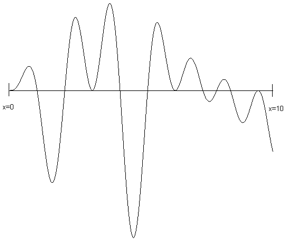
For a sample problem, let’s suppose that we want to find the maximum value of the function F with one independent variable x in the following equation and as seen in last figure:
F(x) = sin(x) * sin(0.4 * x) * sin(3 * x)
The problem that we want to solve is finding a good value of x to find a near to possible maximum value of F(x). To be clear: we encode a floating point number as a chromosome made up of a specific number of bits so any chromosome with randomly set bits will represent some random number in the interval [0, 10]. The fitness function is simply the function in the last equation.
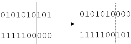
This figure shows an example of a crossover operation that we will implement later in the program example. A random chromosome bit index is chosen, and two chromosomes are “cut” at this index and swap cut parts. The two original chromosomes in generation_n are shown on the left of the figure and after the crossover operation they produce two new chromosomes in generation n + 1 where n is the current generation number. The two new chromosomes are shown on the right of the figure.
In addition to using crossover operations to create new chromosomes from existing chromosomes, we will also perform genetic mutation by randomly flipping bits in chromosomes. A fitness function that rates the fitness value of each chromosome allows us to decide which chromosomes to discard and which to use for the next generation. We will use the most fit chromosomes in the population for producing the next generation using crossover and mutation.
We will implement a general purpose Java GA library in the next section and then solve the example problem posed at the end of this chapter in the GA Example Section.
Java Library for Genetic Algorithms
The full implementation of the GA library is in the Java source file Genetic.java. The following code snippets show the method signatures defining the public API for the library. Note that there are two constructors, the first using default values for the fraction of chromosomes on which to perform crossover and mutation operations and the second constructor allows setting explicit values for these parameters:
    abstract public class Genetic {
      public Genetic(int num_genes_per_chromosome,
                     int num_chromosomes)
      public Genetic(int num_genes_per_chromosome,
                     int num_chromosomes,
                     float crossover_fraction,
                     float mutation_fraction)
The method sort is used to sort the population of chromosomes in most fit first order. The methods getGene and setGene are used to fetch and change the value of any gene (bit) in any chromosome. These methods are protected because you may need to override them in derived classes.
      protected void sort()
      protected boolean getGene(int chromosome,
                                int gene)
      protected void setGene(int chromosome,
                             int gene, int value)
      protected void setGene(int chromosome,
                             int gene,
                             boolean value)
The methods evolve, doCrossovers, doMutations, and doRemoveDuplicates are utilities for running GA simulations. These methods are protected but you will probably not need to override them in derived classes.
      protected void evolve()
      protected void doCrossovers()
      protected void doMutations()
      protected void doRemoveDuplicates()
When you subclass class Genetic you must implement the following abstract method calcFitness that will determine the evolution of chromosomes during the GA simulation.
      // Implement the following method in sub-classes:
      abstract public void calcFitness();
    }
The class Chromosome represents an ordered bit sequence with a specified number of bits and a floating point fitness value.
    class Chromosome {
      private Chromosome()
      public Chromosome(int num_genes)
      public boolean getBit(int index)
      public void setBit(int index, boolean value)
      public float getFitness()
      public void setFitness(float value)
      public boolean equals(Chromosome c)
    }
The class ChromosomeComparator implements a Comparator interface and is application specific. It is used to sort a population in “best first” order:
    class ChromosomeComparator
          implements Comparator<Chromosome> {
      public int compare(Chromosome o1,
                         Chromosome o2)
    }
The last class ChromosomeComparator is used when using the Java Collection class static sort method.
The class Genetic is an abstract class: you must subclass it and implement the method calcFitness that uses an application specific fitness function (that you must supply) to set a fitness value for each chromosome.
The following UML class diagram provides an overview of the Java classes and their public APIs as well as the class MyGenetic that will implement a fitness function for our example of finding a maximum value in an equation and the test class TestGenetic:
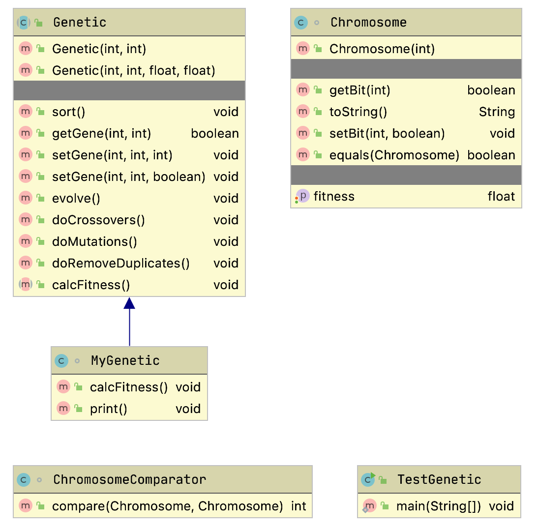
This GA library provides the following behavior:
- Generates an initial random population with a specified number of bits (or genes) per chromosome and a specified number of chromosomes in the population
- Ability to evaluate each chromosome based on a numeric fitness function
- Ability to create new chromosomes from the most fit chromosomes in the population using the genetic crossover and mutation operations
There are two class constructors for Genetic set up a new GA experiment. Both constructors require the number of genes (or bits) per chromosome, and the number of chromosomes in the population. The second constructor allows you to optionally set the fractions for mutation and crossover operations.
The Genetic class constructors build an array of integers rouletteWheel which is used to weight the most fit chromosomes in the population for choosing the parents of crossover and mutation operations. When a chromosome is being chosen, a random integer is selected to be used as an index into the rouletteWheel array; the values in the array are all integer indices into the chromosome array. More fit chromosomes are heavily weighted in favor of being chosen as parents for the crossover operations. The algorithm for the crossover operation is fairly simple; here is the implementation:
     public void doCrossovers() {
       int num = (int)(numChromosomes * crossoverFraction);
       for (int i = num - 1; i >= 0; i--) {
         // Don't overwrite the "best" chromosome
         // from current generation:
         int c1 = 1 + (int) ((rouletteWheelSize - 1) *
                             Math.random() * 0.9999f);
         int c2 = 1 + (int) ((rouletteWheelSize - 1) *
                             Math.random() * 0.9999f);
         c1 = rouletteWheel[c1];
         c2 = rouletteWheel[c2];
         if (c1 != c2) {
           int locus = 1+(int)((numGenesPerChromosome-2) *
                               Math.random());
           for (int g = 0; g<numGenesPerChromosome; g++) {
             if (g < locus) {
               setGene(i, g, getGene(c1, g));
             } else {
               setGene(i, g, getGene(c2, g));
             }
           }
         }
       }
     }
The method doMutations is similar to doCrossovers: we randomly choose chromosomes from the population and for these selected chromosomes we randomly “flip” the value of one gene (a gene is a bit in our implementation):
      public void doMutations() {
        int num = (int)(numChromosomes * mutationFraction);
        for (int i = 0; i < num; i++) {
          // Don't overwrite the "best" chromosome
          // from current generation:
          int c = 1 + (int) ((numChromosomes - 1) *
                             Math.random() * 0.99);
          int g = (int) (numGenesPerChromosome *
                         Math.random() * 0.99);
          setGene(c, g, !getGene(c, g));
        }
      }
We developed a general purpose library in this section for simulating populations of chromosomes that can evolve to a more “fit” population given a fitness function that ranks individual chromosomes in order of fitness. In the next section we will develop an example GA application by defining the size of a population and the fitness function that we saw earlier.
Finding the Maximum Value of a Function
We will use the Java library in the last section to develop an example application to find the maximum of the function seen in the figure showing the sample function which shows a plot of our test function we are using a GA to fit, plotted in the interval [0, 10].
While we could find the maximum value of this function by using Newton’s method (or even a simple brute force search over the range of the independent variable x), the GA method scales very well to similar problems of higher dimensionality. The GA also helps us to find better than locally optimum solutions. In this example we are working in one dimension so we only need to encode a single variable in a chromosome. As an example of a 20-dimensional space, we might have a financial model with 20 independent variables x1, x2, ..x20 and a single chromosome would still represent a point in this 20-dimensional space. To continue this example, if we used 10 bits to represent the value range in each of the 20 dimensions, then the chromosome would be represented as 200 bits.
To generalize, our first task is to characterize the search space as one or more parameters. In general when we write GA applications we might need to encode several parameters in a single chromosome. As another example, if a fitness function has three arguments we would encode three numbers in a single chromosome.
Let’s get back to our 1-dimensional example seen in the figure showing the sample function. This is a simple example showing you how to set up a GA simulation. In this example problem we have only one parameter, the independent variable x. We will encode the parameter x using ten bits (so we have ten 1-bit genes per chromosome). A good starting place is writing a utility method for converting the 10-bit representation to a floating-point number in the range [0.0, 10.0]:
    float geneToFloat(int chromosomeIndex) {
      int base = 1;
      float x = 0;
      for (int j=0; j<numGenesPerChromosome; j++)  {
         if (getGene(chromosomeIndex, j)) {
            x += base;
         }
         base *= 2;
      }
For each bit at index j with a value of 1, add \(2 ^j\) to the sum x. We need to normalize this sum x that is an integer in the range of [0,1023] to a floating point number in the approximate range of [0, 10]:
      x /= 102.4f;
      return x;
    }
Note that we do not need the reverse method! We use our GA library from the last section to create a population of 10-bit chromosomes. In order to evaluate the fitness of each chromosome in a population, we only have to convert the 10-bit representation to a floating-point number for evaluation using the fitness function we showed earlier (figure showing the sample function):
    private float fitness(float x) {
      return (float)(Math.sin(x) *
                     Math.sin(0.4f * x) *
                     Math.sin(3.0f * x));
    }
The following table shows some sample random chromosomes and the floating point numbers that they encode. The first column shows the gene indices where the bit is “on,” the second column shows the chromosomes as an integer number represented in binary notation, and the third column shows the floating point number that the chromosome encodes. Note that the center column in the following table shows the bits in order where index 0 is the left-most bit, and index 9 is the right-most bit; this is the reverse of the normal order for encoding integers but the GA does not care, it works with any encoding we use as long as it is consistent.
Using methods geneToFloat and fitness we now implement the abstract method calcFitness from our GA library class Genetic so the derived class TestGenetic is not abstract. This method has the responsibility for calculating and setting the fitness value for every chromosome stored in an instance of class Genetic:
    public void calcFitness() {
      for (int i=0; i<numChromosomes; i++) {
        float x = geneToFloat(i);
        chromosomes.get(i).setFitness(fitness(x));
      }
    }
While it was useful to make this example more clear with a separate geneToFloat method, it would have also been reasonable to simply place the formula in the method fitness in the implementation of the abstract (in the base class) method calcFitness.
In any case we are done with coding this example. You can compile the two example Java files Genetic.java and TestGenetic.java, and run the TestGenetic class to verify that the example program quickly finds a near maximum value for this function. The project Makefile has a single target that builds the library and runs the example test program:
test:
 mvn install
 mvn exec:java -Dexec.mainClass="com.markwatson.geneticalgorithm.TestGenetic"
You can try setting different numbers of chromosomes in the population and try setting non-default crossover rates of 0.85 and a mutation rates of 0.3. We will look at a run with a small number of chromosomes in the population created with:
      genetic_experiment =
                     new MyGenetic(10, 20, 0.85f, 0.3f);
      int NUM_CYCLES = 500;
      for (int i=0; i<NUM_CYCLES; i++) {
        genetic_experiment.evolve();
        if ((i%(NUM_CYCLES/5))==0 || i==(NUM_CYCLES-1)) {
          System.out.println("Generation " + i);
          genetic_experiment.print();
        }
      }
In this experiment 85% of chromosomes will be “sliced and diced” with a crossover operation and 30% will have one of their genes changed. We specified 10 bits per chromosome and a population size of 20 chromosomes. In this example, I have run 500 evolutionary cycles. After you determine a fitness function to use, you will probably need to experiment with the size of the population and the crossover and mutation rates. Since the simulation uses random numbers (and is thus non-deterministic), you can get different results by simply rerunning the simulation. Here is example program output (with much of the output removed for brevity):
    count of slots in roulette wheel=55
    Generation 0
    Fitness for chromosome 0 is 0.505, occurs at x=7.960
    Fitness for chromosome 1 is 0.461, occurs at x=3.945
    Fitness for chromosome 2 is 0.374, occurs at x=7.211
    Fitness for chromosome 3 is 0.304, occurs at x=3.929
    Fitness for chromosome 4 is 0.231, occurs at x=5.375
    ...
    Fitness for chromosome 18 is -0.282 occurs at x=1.265
    Fitness for chromosome 19 is -0.495, occurs at x=5.281
    Average fitness=0.090 and best fitness for this
    generation:0.505
    ...
    Generation 499
    Fitness for chromosome 0 is 0.561, occurs at x=3.812
    Fitness for chromosome 1 is 0.559, occurs at x=3.703
    ...
This example is simple but is intended to show you how to encode parameters for a problem where you want to search for values to maximize a fitness function that you specify. Using the library developed in this chapter you should be able to set up and run a GA simulation for your own applications.
The important takeaway is that if you can encode a problem space as a chromosome and you have a fitness function to rate the numerical effectiveness of a chromosome, then Genetic Algorithms are an effective alternative to greedy search algorithms.
Neural Networks
In a sense training neural networks is a search problem. Given training data and using gradient descent we search for a set of parameters (the weights in a neural network) that model the training data. A dataset is defined by the features in the dataset and the data samples. If we consider our search space to have a number of dimensions equal to the number of features then we can at least imagine that the training samples are an extremely sparse scattering of points in this high-dimensional space. These training data are a distribution of the possible points in this space. Since input features are often correlated we would not expect an even distribution of samples over this space. We refer to the training samples as being “in distribution” and new data that we later process with our trained model to be “out of distribution.” New “out of distribution” data may sometimes represent areas of the space with no training examples nearby and we would expect our model to sometimes perform poorly on this data.
Neural networks can be used to efficiently solve many problems that are intractable or difficult using other AI programming techniques. In the late 1980s I spent almost two years on a DARPA neural network tools advisory panel, wrote the ANSim neural network product, and have used neural networks for a wide range of application problems (radar interpretation, bomb detection, and as controllers in computer games). Mastering the use of neural networks will allow you to solve many types of problems that are very difficult to solve using other methods.
Gradient descent is a general term for moving in a direction in a space that is “down hill” towards a local minimum. Here I write an implementation for a backpropagation neural network from scratch (pure Java code, no libraries). The material in this chapter is meant to provide you with an intuition of how backpropagation works while the next chapter covers a robust deep learning library that you should use in for modeling large datasets. Backpropagation is a type of gradient descent that works by changing weight values (the parameters in a neural network model) in the direction of reducing the error between what our model predicts for a set of input values and what the target output is in training data.
In the next chapter Deep Learning Using Deeplearning4j we will use a popular Java deep learning library that can efficiently process neural networks with more complex architectures and larger numbers of simulated neurons. These “Deep Learning” neural networks use computational tricks to efficiently train more complex Backpropagation networks.
Although most of this book is intended to provide practical advice (with some theoretical background) on using AI programming techniques, I cannot imagine being interested in practical AI programming without also thinking about the philosophy and mechanics of how the human mind works. I hope that my readers share this interest.
The physical structure and dynamics of the human brain are inherently parallel and distributed [Parallel Distributed Processing: Explorations in the Microstructure of Cognition, Rumelhart, McClelland, etc. 1986]. We are experts at doing many things at once. For example, I simultaneously can walk, talk with my wife, keep our puppy out of cactus, and enjoy the scenery behind our house in Sedona, Arizona. AI software systems struggle to perform even narrowly defined tasks well, so how is it that we are able to simultaneously perform several complex tasks? There is no clear or certain answer to this question at this time, but certainly the distributed neural architecture of our brains is a requirement for our abilities. Classical artificial neural network simulations (like the ones we study in this chapter) do not address “multi-tasking” (other techniques that do address this issue are multi-agent systems with some form or mediation between agents). Deep learning models can have multiple types of inputs, different types of outputs, and complex internal structure - basically connected models that are trained jointly. While deep learning models trained jointly on different types of input data break through the limitations of simple backpropagation models, the simple backpropagation models we look at now are still very practical today for a range of problems.
Also interesting is the distinction between instinctual behavior and learned behavior. Our knowledge of GAs from the chapter on Genetic Algorithms provides a clue to how the brains of lower order animals can be hardwired to provide efficient instinctual behavior under the pressures of evolutionary forces (i.e., likely survival of more fit individuals). This works by using genetic algorithms to design specific neural wiring. I have used genetic algorithms to evolve recurrent neural networks for control applications (I wrote about this in C++ Power Paradigms, 1995, McGraw-Hill). This work had only partial success but did convince me that biological genetic pressure is probably adequate to “pre-wire” some forms of behavior in natural (biological) neural networks.
While we will study supervised learning techniques in this chapter, it is possible to evolve both structure and attributes of neural networks using other types of neural network models like Adaptive Resonance Theory (ART) to autonomously learn to classify learning examples without intervention.
We will start this chapter by discussing human neuron cells and which features of real neurons that we will model. Unfortunately, we do not yet understand all of the biochemical processes that occur in neurons, but there are fairly accurate models available (web search “neuron biochemical”). Neurons are surrounded by thin hair-like structures called dendrites which serve to accept activation from other neurons. Neurons sum up activation from their dendrites and each neuron has a threshold value; if the activation summed over all incoming dendrites exceeds this threshold, then the neuron fires, spreading its activation to other neurons. Dendrites are very localized around a neuron. Output from a neuron is carried by an axon, which is thicker than dendrites and potentially much longer than dendrites in order to affect remote neurons. The following figure shows the physical structure of a neuron; in general, the neuron’s axon would be much longer than is seen in this figure. The axon terminal buttons transfer activation to the dendrites of neurons that are close to the individual button. An individual neuron is connected to up to ten thousand other neurons in this way.
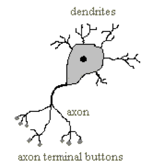
The activation absorbed through dendrites is summed together, but the firing of a neuron only occurs when a threshold is passed. In neural network simulations there are several common ways to model neurons and connections between neurons that we will see in both this and the next chapter.
Road Map for the Neural Network Example Code
The following UML class diagram will give you an overview all of the neural network library classes in this chapter before we dive into the code:
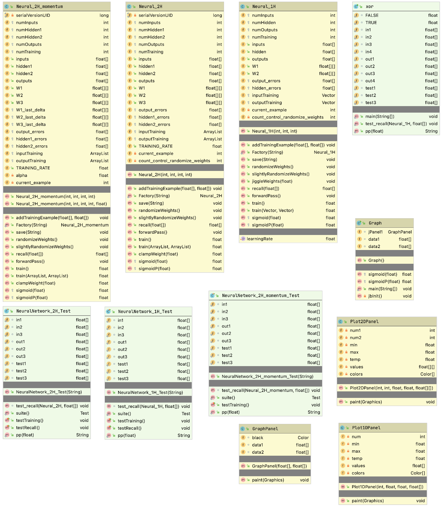
There are three parts to the code base: main backpropagation library, GUI examples, and text-only tests. The following screen show of the project open in an IDE is useful to see the file layout for the project:

Backpropagation Neural Networks
The neural network model that we use is called backpropagation, also known as back-prop or delta rule learning. In this model, neurons are organized into data structures that we call layers. The figure Backpropagation network with No Hidden Layer shows a simple neural network with two layers; this network is shown in two different views: just the neurons organized as two one-dimensional arrays, and as two one-dimensional arrays with the connections between the neurons. In our model, there is a connection between two neurons that is characterized by a single floating-point number that we will call the connection’s weight. A weight W_{i,j} connects input neuron i to output neuron j. In the back propagation model, we always assume that a neuron is connected to every neuron in the previous layer.
A key feature of back-prop neural networks is that they can be efficiently trained. Training is performed by calculating sets of weights for connecting each layer. As we will see, we will train networks by applying input values to the input layer, allowing these values to propagate through the network using the current weight values, and calculating the errors between desired output values and the output values from propagation of input values through the network.
The errors at the output layer are used to calculate gradients (or corrections) to the weights feeding into the output layer. Gradients are back propagated through the network allowing all weights in the network to be updated to reduce errors visible at the output layer.
One limitation of early back propagation neural networks is that they are limited to the number of neuron layers that can be efficiently trained. More recent advances in deep learning have mostly solved this problem: as error gradients are back propagated through the network toward the input layer, the gradients get smaller and smaller. If these gradients vanish because they can’t be represented as a floating point number then weight updates will be zero and the model is not trained. Another effect of many hidden layers is that it can take a lot of time to train back propagation networks. This problem has also mostly been solved with modern deep learning libraries as seen in the next chapter Deep Learning.
Initially, weights are set to small random values. You will get a general idea for how this is done in this section and then we will look at Java implementation code in the section for a Java Class Library for Backpropagation.
In the figure showing a Backpropagation network with No Hidden Layer, we have only two neuron layers, one for the input neurons and one for the output neurons. Networks with no hidden layers are not generally useful - I am using the network in the figure showing a Backpropagation network with No Hidden Layer just to demonstrate layer to layer connections through a weights array.
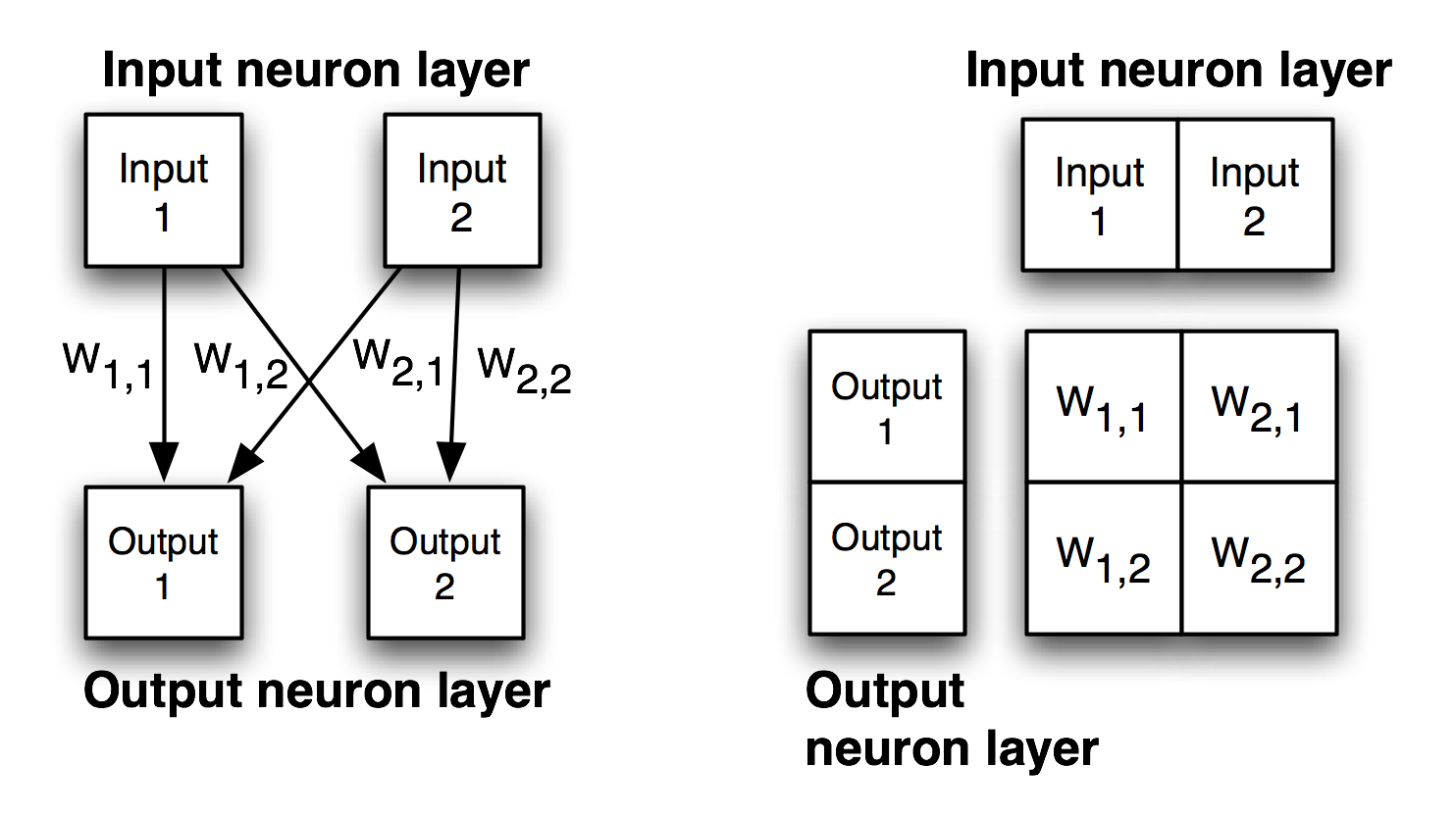
To calculate the activation of the first output neuron O1, we evaluate the sum of the products of the input neurons times the appropriate weight values; this sum is input to a Sigmoid activation function (see the figure showing the Sigmoid Function) and the result is the new activation value for O1. Here is the formula for the simple network in the figure showing a Backpropagation network with No Hidden Layer:
O1 = Sigmoid (I1 * W[1,1] + I2 * W[2,1])
O2 = Sigmoid (I2 * W[1,2] + I2 * W[2,2])
The figure showing the Sigmoid Function shows a plot of the Sigmoid function and the derivative of the sigmoid function (SigmoidP). We will use the derivative of the Sigmoid function when training a neural network (with at least one hidden neuron layer) with classified data examples.
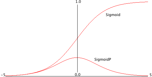
A neural network like the one seen in the figure showing a Backpropagation network with No Hidden Layer is trained by using a set of training data. For back propagation networks, training data consists of matched sets of input with matching desired output values. We want to train a network to not only produce similar outputs for training data inputs as appear in the training data, but also to generalize its pattern matching ability based on the training data to be able to match test patterns that are similar to training input patterns. A key here is to balance the size of the network against how much information it must hold. A common mistake when using back-prop networks is to use too large a network: a network that contains too many neurons and connections will simply memorize the training examples, including any noise in the training data. However, if we use a smaller number of neurons with a very large number of training data examples, then we force the network to generalize, ignoring noise in the training data and learning to recognize important traits in input data while ignoring statistical noise.
How do we train a back propagation neural network given that we have a good training data set? The algorithm is quite easy; we will now walk through the simple case of a two-layer network like the one in the figure showing a Backpropagation network with No Hidden Layer. Later in the section for a Java Class Library for Back Propagation we will review the algorithm in more detail when we have either one or two hidden neuron layers between the input and output layers.
In order to train the network in the figure for a Backpropagation network with No Hidden Layer, we repeat the following learning cycle several times:
- Zero out temporary arrays for holding the error at each neuron. The error, starting at the output layer, is the difference between the output value for a specific output layer neuron and the calculated value from setting the input layer neuron’s activation values to the input values in the current training example, and letting activation spread through the network.
- Update the weight W_{i,j} (where i is the index of an input neuron, and j is the index of an output neuron) using the formula W_{i,j} += learning_rate * output_error_j*I_i (learning_rate is a tunable parameter) and output_error_j was calculated in step 1, and I_i is the activation of input neuron at index i.
This process is continued to either a maximum number of learning cycles or until the calculated output errors get very small. We will see later that the algorithm is similar but slightly more complicated when we have hidden neuron layers; the difference is that we will “back propagate” output errors to the hidden layers in order to estimate errors for hidden neurons. We will cover more on this later. This type of neural network is too simple to solve very many interesting problems, and in practical applications we almost always use either one additional hidden neuron layer or two additional hidden neuron layers. The figure showing mappings supported by zero hidden layer, one hidden layer, and two hidden hidden layer networks shows the types of problems that can be solved by networks with different numbers of hidden layers.
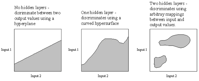
A Java Class Library for Back Propagation
The back propagation neural network library used in this chapter was written to be easily understood and is useful for many problems. However, one thing that is not in the implementation in this section (it is added in the section Using Momentum to speed up training) is something usually called “momentum” to speed up the training process at a cost of doubling the storage requirements for weights. Adding a “momentum” term not only makes learning faster but also increases the chances of successfully learning more difficult problems.
We will concentrate in this section on implementing a back-prop learning algorithm that works for both one and two hidden layer networks. As we saw in the Figure showing mappings supported by zero hidden layer, one hidden layer, and two hidden layer networks, a network with two hidden layers is capable of arbitrary mappings of input to output values. It used to be a common (and incorrect) opinion that there was no theoretical reason for using networks with three hidden layers. With recent projects using Deep Learning as I mentioned at the beginning of this chapter, neural networks with many hidden layers are now common practice. Here is one of the example programs that helps visualize a 1\one hidden layer network:
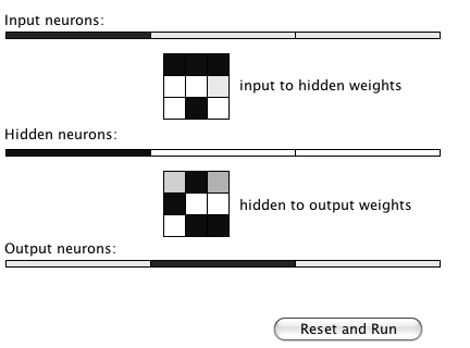
With each layer having three neurons, the weight matrices are 3 x 3 arrays and are easy to display. When you run the examples you can see the weight matches changing in time. Here is another example program that adds an additional hidden layer:
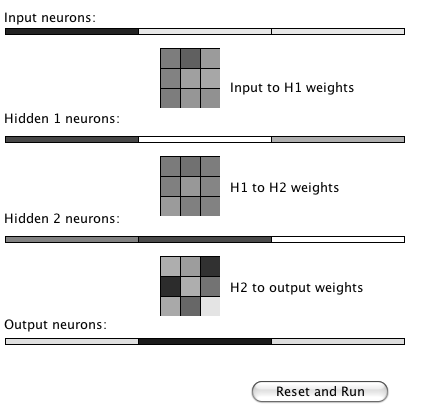
Please note, dear reader, that simple networks like these examples are explainable in the sense that you can understand how they work after they are trained because they have so few parameters. We can characterize the complexity of models as the number of layers and the total number of connection weights. We might say that the one hidden layer model has 9 parameters and the two hidden layer model has 18 parameters (i.e., the total number of weights that we must learn effective values for). In general large neural models, especially deep learning models, are not explainable. There are some applications that are required by law to be explainable for which neural networks are not appropriate to use. Another issue is fairness of models if they are trained on biased data.
The relevant files for the back propagation examples are:
- Neural_1H.java - contains a class for simulating a neural network with one hidden neuron layer
- Test_1H.java - a text-based test program for the class Neural_1H
- GUITest_1H.java - a GUI-based test program for the class Neural_1H
- Neural_2H.java - contains a class for simulating a neural network with two hidden neuron layers
- Neural_2H_momentum.java - contains a class for simulating a neural network with two hidden neuron layers and implements momentum learning (implemented in the section Using Momentum to speed up training
- Test_2H.java - a text-based test program for the class Neural_2H
- GUITest_2H.java - a GUI-based test program for the class Neural_2H
- GUITest_2H_momentum.java - a GUI-based test program for the class Neural_2H_momentum that uses momentum learning (implemented in the section Using Momentum to speed up training
- Plot1DPanel - a Java JFC graphics panel for the values of a one-dimensional array of floating point values
- Plot2DPanel - a Java JFC graphics panel for the values of a two-dimensional array of floating point values
The GUI files are for demonstration purposes only, and we will not discuss the code for these classes; if you are interested in the demo graphics code and do not know JFC Java programming, there are a few good JFC tutorials at the web.
It is common to implement back-prop libraries to handle either zero, one, or two hidden layers in the same code base. At the risk of having to repeat similar code in two different classes, I decided to make the Neural_1H and Neural_2H classes distinct. I think that this makes the code a little easier to understand. As a practical point, you will almost always start solving a neural network problem using only one hidden layer and only progress to trying two hidden layers if you can’t train a one hidden layer network to solve the problem at-hand with sufficiently small error when tested with data that is different from the original training data. Networks with only one hidden layer require less storage space and run faster in simulation than two hidden layer networks.
In this section we will look only at the implementation of the class Neural_2H (class Neural_1H is simpler and when you understand how Neural_2H works, the simpler class is also easy to understand). This class implements the Serializable interface and contains a utility method save to write a trained network to a disk file:
class Neural_2H implements Serializable {
There is a static factory method that reads a saved network file from disk and builds an instance of Neural_2H and there is a class constructor that builds a new untrained network in memory, given the number of neurons in each layer:
     public static Neural_2H Factory(String serialized_file_name)
     public Neural_2H(int num_in,
                      int num_hidden1,
                      int num_hidden2, int num_output)
An instance of Neural_2H contains training data as transient data that is not saved by method save.
     transient protected ArrayList inputTraining = new Vector();
     transient protected ArrayList outputTraining = new Vector();
I want the training examples to be native float arrays so I used generic ArrayList containers. You will usually need to experiment with training parameters in order to solve difficult problems. The learning rate not only controls how large the weight corrections we make each learning cycle but this parameter also affects whether we can break out of local minimum. Other parameters that affect learning are the ranges of initial random weight values that are hardwired in the method randomizeWeights() and the small random values that we add to weights during the training cycles; these values are set in in slightlyRandomizeWeights(). I usually only need to adjust the learning rate when training back-prop networks:
public float TRAINING_RATE = 0.5f;
I often decrease the learning rate during training - that is, I start with a large learning rate and gradually reduce it during training. The calculation for output neuron values given a set of inputs and the current weight values is simple. I placed the code for calculating a forward pass through the network in a separate method forwardPass() because it is also used later in the method training:
     public float[] recall(float[] in) {
       for (int i = 0; i < numInputs; i++) inputs[i] = in[i];
       forwardPass();
       float[] ret = new float[numOutputs];
       for (int i = 0; i < numOutputs; i++) ret[i] = outputs[i];
       return ret;
     }

     public void forwardPass() {
       for (int h = 0; h < numHidden1; h++) {
         hidden1[h] = 0.0f;
       }
       for (int h = 0; h < numHidden2; h++) {
         hidden2[h] = 0.0f;
       }
       for (int i = 0; i < numInputs; i++) {
         for (int h = 0; h < numHidden1; h++) {
           hidden1[h] += inputs[i] * W1[i][h];
         }
       }
       for (int i = 0; i < numHidden1; i++) {
         for (int h = 0; h < numHidden2; h++) {
           hidden2[h] += hidden1[i] * W2[i][h];
         }
       }
       for (int o = 0; o < numOutputs; o++) outputs[o] = 0.0f;
       for (int h = 0; h < numHidden2; h++) {
         for (int o = 0; o < numOutputs; o++) {
           outputs[o] += sigmoid(hidden2[h]) * W3[h][o];
         }
       }
     }
While the code for recall and forwardPass is almost trivial, the training code in method train is more complex and we will go through it in some detail. Before we get to the code, I want to mention that there are two primary techniques for training back-prop networks. The technique that I use is to update the weight arrays after each individual training example. The other technique is to sum all output errors over the entire training set (or part of the training set) and then calculate weight updates. In the following discussion, I am going to weave my comments on the code into the listing. The private member variable current_example is used to cycle through the training examples: one training example is processed each time that the train method is called:
     private int current_example = 0;

     public float train(ArrayList ins, ArrayList v_outs) {
Before starting a training cycle for one example, we zero out the arrays used to hold the output layer errors and the errors that are back propagated to the hidden layers. We also need to copy the training example input values and output values:
     int i, h, o; float error = 0.0f;
     int num_cases = ins.size();
     for (int example=0; example<num_cases; example++) {
       // zero out error arrays:
       for (h = 0; h < numHidden1; h++) hidden1_errors[h] = 0.0f;
       for (h = 0; h < numHidden2; h++) hidden2_errors[h] = 0.0f;
       for (o = 0; o < numOutputs; o++) output_errors[o] = 0.0f;
       // copy the input values:
       for (i = 0; i < numInputs; i++) {
         inputs[i] = ((float[]) ins.get(current_example))[i];
       }
       // copy the output values:
       float[] outs = (float[]) v_outs.get(current_example);
We need to propagate the training example input values through the hidden layers to the output layers. We use the current values of the weights:
forwardPass();
After propagating the input values to the output layer, we need to calculate the output error for each output neuron. This error is the difference between the desired output and the calculated output; this difference is multiplied by the value of the calculated output neuron value that is first modified by the Sigmoid function that we saw in the figure showing the Sigmoid Function. The Sigmoid function is to clamp the calculated output value to a reasonable range.
     for (o = 0; o < numOutputs; o++) {
       output_errors[o] = (outs[o] - outputs[o]) * sigmoidP(outputs[o]);
     }
The errors for the neuron activation values in the second hidden layer (the hidden layer connected to the output layer) are estimated by summing for each hidden neuron its contribution to the errors of the output layer neurons. The thing to notice is that if the connection weight value between hidden neuron h and output neuron o is large, then hidden neuron h is contributing more to the error of output neuron o than other neurons with smaller connecting weight values:
     for (h = 0; h < numHidden2; h++) {
       hidden2_errors[h] = 0.0f; for (o = 0; o < numOutputs; o++) {
         hidden2_errors[h] += output_errors[o] * W3[h][o];
       }
     }
We estimate the errors in activation energy for the first hidden layer neurons by using the estimated errors for the second hidden layers that we calculated in the last code snippet:
     for (h = 0; h < numHidden1; h++) {
       hidden1_errors[h] = 0.0f; for (o = 0; o < numHidden2; o++) {
         hidden1_errors[h] += hidden2_errors[o] * W2[h][o];
       }
     }
After we have scaled estimates for the activation energy errors for both hidden layers we then want to scale the error estimates using the derivative of the sigmoid function’s value of each hidden neuron’s activation energy:
     for (h = 0; h < numHidden2; h++) {
       hidden2_errors[h] = hidden2_errors[h] * sigmoidP(hidden2[h]);
     }
     for (h = 0; h < numHidden1; h++) {
       hidden1_errors[h] = hidden1_errors[h] * sigmoidP(hidden1[h]);
     }
Now that we have estimates for the hidden layer neuron errors, we update the weights connecting to the output layer and each hidden layer by adding the product of the current learning rate, the estimated error of each weight’s target neuron, and the value of the weight’s source neuron:
     // update the hidden2 to output weights:
     for (o = 0; o < numOutputs; o++) {
       for (h = 0; h < numHidden2; h++) {
         W3[h][o] += TRAINING_RATE * output_errors[o] * hidden2[h];
         W3[h][o] = clampWeight(W3[h][o]);
       }
     }
     // update the hidden1 to hidden2 weights:
     for (o = 0; o < numHidden2; o++) {
       for (h = 0; h < numHidden1; h++) {
         W2[h][o] += TRAINING_RATE * hidden2_errors[o] * hidden1[h];
         W2[h][o] = clampWeight(W2[h][o]);
       }
     }
     // update the input to hidden1 weights:
     for (h = 0; h < numHidden1; h++) {
       for (i = 0; i < numInputs; i++) {
         W1[i][h] += TRAINING_RATE * hidden1_errors[h] * inputs[i];
         W1[i][h] = clampWeight(W1[i][h]);
       }
     }
     for (o = 0; o < numOutputs; o++) {
       error += Math.abs(outs[o] - outputs[o]);
     }
The last step in this code snippet was to calculate an average error over all output neurons for this training example. This is important so that we can track the training status in real time. For very long running back-prop training experiments I like to be able to see this error graphed in real time to help decide when to stop a training run. This allows me to experiment with the learning rate initial value and see how fast it decays. The last thing that method train needs to do is to update the training example counter so that the next example is used the next time that train is called:
     current_example++;
     if (current_example >= num_cases)
       current_example = 0;
     return error;
   }
You can look at the implementation of the Swing GUI test class GUTest_2H to see how I decrease the training rate during training. I also monitor the summed error rate over all output neurons and occasionally randomize the weights if the network is not converging to a solution to the current problem.
Adding Momentum to Speed Up Back-Prop Training
We did not use a momentum term in the Java code in the section for a Java Class Library for Back Propagation. For difficult to train problems, adding a momentum term can drastically reduce the training time at a cost of doubling the weight storage requirements. To implement momentum, we remember how much each weight was changed in the previous learning cycle and make the weight change larger if the current change in “direction” is the same as the last learning cycle. For example, if the change to weight W_{i,j} had a large positive value in the last learning cycle and the calculated weight change for W_{i,j} is also a large positive value in the current learning cycle, then make the current weight change even larger. Adding a “momentum” term not only makes learning faster but also increases the chances of successfully learning more difficult problems.
I modified two of the classes from the section for a Java Class Library for Back Propagation to use momentum:
- Neural_2H_momentum.java - training and recall for two hidden layer back-prop networks. The constructor has an extra argument “alpha” that is a scaling factor for how much of the previous cycle’s weight change to add to the new calculated delta weight values.
- GUITest_2H_momentum.java - a GUI test application that tests the new class Neural_2H_momentum.
The code for class Neural_2H_momentum is similar to the code for Neural_2H that we saw in the last section so here we will just look at the differences. The class constructor now takes another parameter alpha that determines how strong the momentum correction is when we modify weight values:
     // momentum scaling term that is applied
     // to last delta weight:
     private float alpha = 0.2f;
While this alpha term is used three times in the training code, it suffices to just look at one of these uses in detail. When we allocated the three weight arrays W1, W2, and W3 we also now allocate three additional arrays of corresponding same size: W1_last_delta, W2_last_delta, and W3_last_delta. These three new arrays are used to store the weight changes for use in the next training cycle. Here is the original code to update W3 from the last section:
W3[h][o] += TRAINING_RATE * output_errors[o] * hidden2[h];
The following code snippet shows the additions required to use momentum:
     W3[h][o] += TRAINING_RATE * output_errors[o] * hidden2[h] +
       // apply the momentum term:
       alpha * W3_last_delta[h][o];
     W3_last_delta[h][o] = TRAINING_RATE * output_errors[o] * hidden2[h];
I mentioned in the last section that there are at least two techniques for training back-prop networks: updating the weights after processing each training example or waiting to update weights until all training examples are processed. I always use the first method when I don’t use momentum. In many cases it is best to use the second method when using momentum. In the next chapter on Deep Learning we use a third method for using training data: we choose randomly selected small batches of training examples for each weight update cycle.
Wrap-up for Neural Networks
I hope that the material in this chapter has given you some low-level understanding of the implementation of backpropagation neural networks. We will use a popular deep learning library in the next chapter that in practice you should prefer to the pedantic code here. That said, I used very similar C++ code to that developed here for several practical engineering problems in the 1980s and early 1990s including the prediction code for a bomb detector my company made for the FAA.
Deep Learning Using Deeplearning4j
One limitation of back propagation neural networks seen in the last chapter is that they are limited to the number of neuron layers that can be efficiently trained. If you experimented with the sample back propagation code then you may have noticed that it took longer to train a network with two hidden layers compared to the training time for a network with only one hidden layer. There are also problems like vanishing gradients (the backpropagated errors that are used to update connection weights) that occur in architectures with many layers. Deep learning uses computational improvements to mitigate the vanishing gradient problem like using ReLu activation functions rather than the more traditional Sigmoid function, and networks called “skip connections” networks where some layers are initially turned off with connections skipping to the next active layer. After some initial training the skipped layers are activated and become part of the model (as in ResNet50, mentioned in the section Roadmap for the DL4J Model Zoo at the end of this chapter).
Digging deeper into the problem of vanishing gradients, the problem with back propagation networks is that as error gradients are back propagated through the network toward the input layer, the gradients get smaller and smaller. The effect is that it can take a lot of time to train back propagation networks with many hidden layers. Even worse, the small backpropagated errors get so small that they cause numerical underflows.
I became interested in deep learning neural networks when I took Geoffrey Hinton’s Neural Network class (a Coursera class, taken summer of 2012) and then for the next seven years most of my professional work involved deep learning. I have used GAN (generative adversarial networks) models for synthesizing numeric spreadsheet data, LSTM (long short term memory) models to synthesize highly structured text data like nested JSON, and for NLP (natural language processing). Several of my 55 US patents use neural network and Deep Learning technology.
The Deeplearning4j.org Java library supports many neural network algorithms including support for Deep Learning (DL). Note that I will often refer to Deeplearning4j as DL4J.
We will first look at a simple example of a feed forward network using the same University of Wisconsin cancer database that we used earlier. Deep learning refers to neural networks with many layers, possibly with weights connecting neurons in non-adjacent layers which makes it possible to model temporal and spacial patterns in data.
There is a separate repository of DL4J examples that you should clone because the last half of this chapter is a general discussion of running the DL4J examples and modifying them for your needs with one additional example using LSTM models.
After the first simple example we then look at how to set up DL4J projects using Maven, and then discuss other types of layer classes that you will likely use in your projects. After learning how to set up and use DL4J and having a roadmap of commonly used layer classes, then you will then be set to work on your own projects.
Feed Forward Classification Networks
Feed forward classification networks are a type of deep neural network that can contain multiple hidden neuron layers. In the example here the adjacent layers are fully connected (all neurons in adjacent layers are connected), as in the examples from the last chapter. The difference here is the use of the DL4J library that is written to scale to large problems and to use GPUs if you have them available.
In general, simpler network architectures are better than unnecessarily complicated architectures. You can start with simple architectures and add layers, different layer types, and parallel models as-needed. For feed forward networks model complexity has two dimensions: the numbers of neurons in hidden layers, and also the number of hidden layers. If you put too many neurons in hidden layers then the training data is effectively memorized and this will hurt performance on data samples not used in training. In practice, I “starve the network” by reducing the number of hidden neurons until the model has reduced accuracy on independent test data. Then I slightly increase the number of neurons in hidden layers. This technique helps avoid models simply memorizing training data.
Feed Forward Example
The following screen shot shows an IntelliJ project (you can use the free community or professional version for the examples in this book) for the example in this chapter:
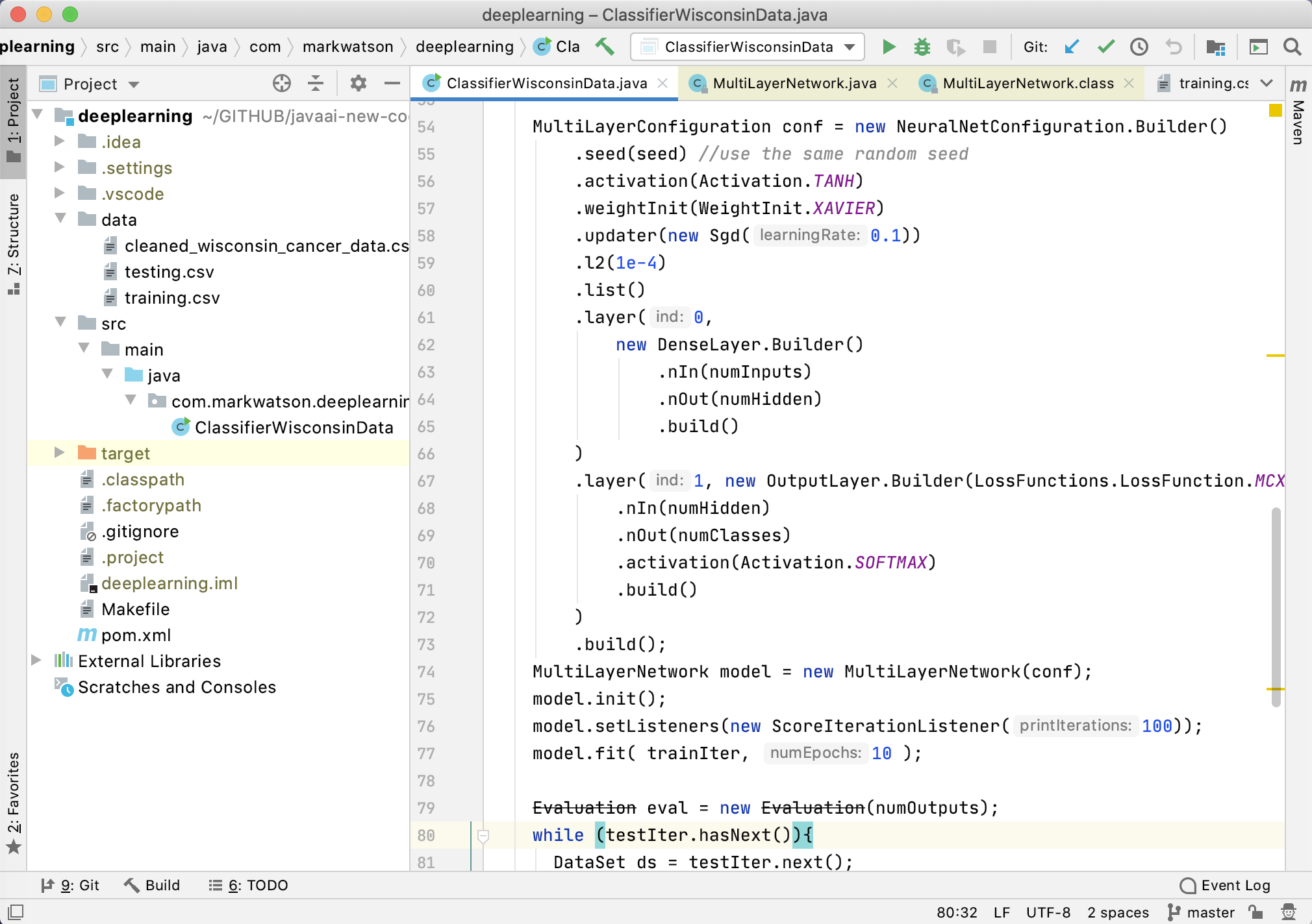
The Deeplearning4j library can use user-written Java classes to import training and testing data into a form that the Deeplearning4j library can use. Some of the examples at https://github.com/eclipse/deeplearning4j-examples use custom data loaders but in this simple example we use built-in utilities for reading spreadsheet data (see lines 46-56 in the following listing).
The class ClassifierWisconsinData reads the University of Wisconsin cancer training and testing data sets, creates a model (lines 59-81), trains it (line 82) and tests it (lines 84-97). The value of the variable numHidden set in line 3 refers to the number of neurons in each hidden layer.
You can increase the number of hidden units in line 36 (something that you might do for more complex problems). To add a hidden layer you can repeat lines 66-71, and you would change the layer indices (first argument) as appropriate in calls to the chained method .layer() so the layer indices are all different and increasing in value.
 1 package com.markwatson.deeplearning;
 2
 3 import org.datavec.api.records.reader.RecordReader;
 4 import org.datavec.api.records.reader.impl.csv.CSVRecordReader;
 5 import org.datavec.api.split.FileSplit;
 6 import org.deeplearning4j.datasets.datavec.RecordReaderDataSetIterator;
 7 import org.deeplearning4j.eval.Evaluation;
 8 import org.deeplearning4j.nn.conf.MultiLayerConfiguration;
 9 import org.deeplearning4j.nn.conf.NeuralNetConfiguration;
10 import org.deeplearning4j.nn.conf.layers.DenseLayer;
11 import org.deeplearning4j.nn.conf.layers.OutputLayer;
12 import org.deeplearning4j.nn.multilayer.MultiLayerNetwork;
13 import org.deeplearning4j.nn.weights.WeightInit;
14 import org.deeplearning4j.optimize.listeners.ScoreIterationListener;
15 import org.nd4j.linalg.activations.Activation;
16 import org.nd4j.linalg.api.ndarray.INDArray;
17 import org.nd4j.linalg.dataset.DataSet;
18 import org.nd4j.linalg.dataset.api.iterator.DataSetIterator;
19 import org.nd4j.linalg.learning.config.Sgd;
20 import org.nd4j.linalg.lossfunctions.LossFunctions;
21 import org.slf4j.Logger;
22 import org.slf4j.LoggerFactory;
23
24 import java.io.*;
25
26 /**
27  * Train a feed forward classifier network on the University of Wisconsin Cancer Dat\
28 a Set.
29  */
30 public class ClassifierWisconsinData {
31
32   private static final Logger log =
33      LoggerFactory.getLogger(ClassifierWisconsinData.class);
34
35   public static void main(String[] args) throws Exception {
36     int numHidden = 3;
37     int numOutputs = 1;
38     int batchSize = 64;
39
40     int seed = 33117;
41
42     int numInputs = 9;
43     int labelIndex = 9;
44     int numClasses = 2;
45
46     RecordReader recordReader = new CSVRecordReader();
47     recordReader.initialize(new FileSplit(new File("data/","training.csv")));
48
49     DataSetIterator trainIter =
50       new RecordReaderDataSetIterator(recordReader,batchSize,labelIndex,numClasses);
51
52     RecordReader recordReaderTest = new CSVRecordReader();
53     recordReaderTest.initialize(
54         new FileSplit(new File("data/","testing.csv")));
55     DataSetIterator testIter =
56         new RecordReaderDataSetIterator(recordReaderTest,batchSize,
57                                     labelIndex,numClasses);
58
59     MultiLayerConfiguration conf = new NeuralNetConfiguration.Builder()
60         .seed(seed) //use the same random seed
61         .activation(Activation.TANH)
62         .weightInit(WeightInit.XAVIER)
63         .updater(new Sgd(0.1))
64         .l2(1e-4)
65         .list()
66         .layer(0,
67             new DenseLayer.Builder()
68                 .nIn(numInputs)
69                 .nOut(numHidden)
70                 .build()
71         )
72         .layer(1, new OutputLayer.Builder(LossFunctions.LossFunction.MCXENT)
73             .nIn(numHidden)
74             .nOut(numClasses)
75             .activation(Activation.SOFTMAX)
76             .build()
77         )
78         .build();
79     MultiLayerNetwork model = new MultiLayerNetwork(conf);
80     model.init();
81     model.setListeners(new ScoreIterationListener(100));
82     model.fit( trainIter, 10 );
83
84     Evaluation eval = new Evaluation(numOutputs);
85     while (testIter.hasNext()) {
86       DataSet ds = testIter.next();
87       INDArray features = ds.getFeatures();
88       System.out.println("Input features: " + features);
89       INDArray labels = ds.getLabels();
90       INDArray predicted = model.output(features,false);
91       System.out.println("Predicted output: "+ predicted);
92       System.out.println("Desired output: "+ labels);
93       eval.eval(labels, predicted);
94       System.out.println();
95     }
96     System.out.println("Evaluate model....");
97     System.out.println(eval.stats());
98   }
99 }
It is very important to not use training data for testing because performance on recognizing training data should always be good assuming that you have enough memory capacity in a network (i.e., enough hidden units and enough neurons in each hidden layer).
The program output is (much output removed for brevity):
The F1 score is calculated as twice precision times recall, divided by precision + recall. We would like F1 to be as close to 1.0 as possible and it is common to spend a fair amount of time experimenting with meta learning parameters to increase F1.
It is also fairly common to try to learn good values of meta learning parameters also. We won’t do this here but the process involves splitting the data into three disjoint sets: training, validation, and testing. The meta parameters are varied, training is performed, and using the validation data the best set of meta parameters is selected. Finally, we test the network as defined by meta parameters and learned weights for those meta parameters with the separate test data to see what the effective F1 score is.
Configuring the Example Using Maven
There is a Maven pom.xml configuration file for this example that is configured for a recent version of DL4J (as I write this in July 2020). DL4J is fairly good at detecting if the Open BLAS library is available, if CUDA software support for any GPUs on your system are available, etc. If you try running the Makefile and get any errors, then check the DL4J Quickstart and setup guide to see if there are any dependencies that you need on your system. The Makefile has a single target:
deep_wisconsin:
  mvn install
  mvn exec:java \
    -Dexec.mainClass="com.markwatson.deeplearning.ClassifierWisconsinData"
Documentation for Other Types of Deep Learning Layers
The documentation for the built-in layer classes in DL4J is probably more than you need for now so let’s review the most other types of layers that I sometimes use. In the simple example we used in the last section we used two types of layers:
- org.deeplearning4j.nn.conf.layers.DenseLayer - maintains connections to all neurons in the previous and next layer, or it is “fully connected.”
- org.deeplearning4j.nn.conf.layers.OutputLayer - has built-in behavior for starting the back propagation calculations back through previous layers.
As you build more deep learning enabled applications, depending on what requirements you have, you will likely need to use at least some of the following Dl4J layer classes:
- org.deeplearning4j.nn.conf.layers.AutoEncoder - often used to remove noise from data. Autoencoders work by making the target training output values equal to the input training values while reducing the number of neurons in the AutoEncoding layer. The layer learns a concise representation of data, or “generalizes” data by learning in which features are important.
- org.deeplearning4j.nn.conf.layers.CapsuleLayer - Capsule networks are an attempt to be more efficient versions of convolutional models. Convolutional networks discard position information of detected features while capsule models maintain and use this information.
- org.deeplearning4j.nn.conf.layers.Convolution1D - one dimensional convolutional layers learn one dimensional feature detectors. Trained layers learn to recognize features but discard the information of where the feature is located. These are often used for data input streams like signal data and word tokens in natural language processing.
- org.deeplearning4j.nn.conf.layers.Convolution2D - two dimensional convolutional layers learn two dimensional feature detectors. Trained layers learn to recognize features but discard the information of where the feature is located. These are often used for recognizing if a type of object appears inside a picture. Note that features, for example representing a nose or a mouth, are recognized but their location in an input picture does not matter. For example, you could cut up an image of someone’s face, moving the ears to the picture center, the mouth to the upper left corner, etc., and the picture would still be predicted to contain a face with some probability because using soft max output layers produces class labels that can be interpreted as probabilities since the values over all output classes sum to the value 1.
- org.deeplearning4j.nn.conf.layers.EmbeddingLayer - embedding layers are used to transform input data into integer data. My most frequent use of embedding layers is word embedding where each word in training data is assigned an integer value. This data can be “one hot encoded” and in the case of processing words, if there are 5000 unique words in the training data for a classifier, then the embedding layer would have 5001 neurons, one for each word and one to represent all words not in the training data. If the word index (indexing is zero-based) is, for example 117, then the activation value for neuron at index 117 is set to one and all others in the layer are set to zero.
- org.deeplearning4j.nn.conf.layers.FeedForwardLayer - this is a super class for most specialized types of feed forward layers so reading through the class reference is recommended.
- org.deeplearning4j.nn.conf.layers.DropoutLayer - dropout layers are very useful for preventing learning new input patterns from making the network forget previously learned patterns. For each training batch, some fraction of neurons in a dropout layer are turned off and don’t update their weights during a training batch cycle. The development of using dropout was key historically for getting deep learning networks to work with many layers and large amounts of training data.
- org.deeplearning4j.nn.conf.layers.LSTM - LSTM layers are used to extend the temporal memory of what a layer can remember. LSTM are a refinement of RNN models that use an input window to pass through a data stream and the RNN model can only use what is inside this temporal sampling window.
- org.deeplearning4j.nn.conf.layers.Pooling1D - a one dimensional pooling layer transforms a longer input to a shorter output by downsampling, i.e., there are fewer output connections than input connections.
- org.deeplearning4j.nn.conf.layers.Pooling2D - a two dimensional pooling layer transforms a larger two dimensional array of data input to a smaller output two dimensional array by downsampling.
Running the DL4J Example Programs and Modifying Them For Your Use
To get started clone the DL4J examples repository written by the authors of DL4J (if you have not already done so) and fetch all of the required libraries:
cd deeplearning4j-examples/dl4j-examples
mvn install
In the next section we will modify Alex Black’s character generating LSTM example for a different application (modeling and generating CSV data). Before moving on to the example in the next section you may want to run his example using:
cd deeplearning4j-examples/dl4j-examples
mvn exec:java -Dexec.mainClass="org.deeplearning4j.examples.advanced.modelling.charm\
odelling.generatetext.GenerateTxtModel"
His example downloads the complete works of Shakespeare from the web and trains a recurrent network LSTM model by passing an input window through the complete text. Each input character is one-hot encoded and the target output is the same one-hot encoded text data in the input window except the sample is shifted one character further in the input text. The model learns to predict the next character in a sequence given a sample of input seed text.
Let’s review one-hot encoding. We need to convert each character in the training data to a one-hot encoding which is a vector of all 0.0 values except for a single value of 1.0. If there are, for example, 256 unique characters in the training data the vector will have 256+1 elements because we add an “unknown character” that represents characters the model may see in the future that are not in the training data. For example if the index of character “m” is 77, then we set element at index 77 to one, all other elements being zero. We won’t look at the implementation of one-hot encoding here because DL4J provides APIs for this. I cover one-hot-encoding implementation in another book in the chapter on Deep Learning for the Hy Language that you can read online.
Here we will be using one-hot encoding for characters but it also works well for encoding words in a vocabulary. Training data may typically have about 10,000 unique words so the one-hot encoding vector would have 10,001 elements. We add a special word position for “unknown word.” For some applications we also use word-embeddings using a smaller vector, 500 elements being a reasonable size. We won’t be using word-embeddings here, or one-hot word embedding but I want you to know what these terms mean.
By processing sufficient sample text, an LSTM network can learn to model the “language” of the input text. If you train on samples from Shakespeare then the model generates text that looks like Shakespeare wrote it. This also works for any author with a specific writing style. LSTM networks are used to model programming languages and many types of structured information.
For a customer, I used an LSTM model trained on JSON log data from AWS. They wanted to have a large amount of test data that did not contain any sensitive information so we generated “fake data” in the correct schema. The LSTM model worked fairly well, the major restriction being that I checked each generated JSON datum for having valid syntax and be valid to the Schema of the original data, discarding samples that failed these tests.
The examples provided with DL4J cover most of the deep learning use cases you may require for your work so I want you to be comfortable running all of the examples and knowing where to start if you want to modify them for a different purposes. If you load the entire DL4J examples repository in a Java IDE and use global search then you should be able to find appropriate CNN, Classification, Regression, etc., examples similar to your current use case that you can modify.
As an experiment, I wanted to try using an LSTM character generation model to generate CSV style spreadsheet data and you can see the implementation of this idea in next section where I modified Alex Black’s character generating LSTM example.
Modifying the Character Generating LSTM Example to Model and Generate CSV Spreadsheet Data
Here are the major changes the I made to the GenerateTxtModel example written by Alex Black. I start by preparing the text training data where I substitute the original method that uses the complete works of William Shakespeare in the class getShakespeareIterator with a new class getWisconsinDataIterator that processes the CSV file in data/training.csv in class LstmCharGenerator:
  static CharacterIterator getWisconsinDataIterator(int miniBatchSize,
                           int sequenceLength)
                 throws IOException {
    String fileLocation = "data/training.csv";
    char[] validCharacters = {'0', '1', '2', '3', '4', '5', '6', '7', '8',
                              '9', ',', '\n'};
    System.out.println("++ valid characters in training data: ");
    for (char ch : validCharacters) System.out.print(" " + ch);
    System.out.println();
    return new CharacterIterator(fileLocation, StandardCharsets.UTF_8,
        miniBatchSize, sequenceLength, validCharacters, new Random(12345));
  }
Changes for configuring the model:
    int lstmLayerSize = 400; //Number of units in each LSTM layer
    int miniBatchSize = 16; //Size of mini batch to use when  training
    int exampleLength = 250;; //Length of each training example sequence to use.
    int tbpttLength = 40; //Length for truncated backpropagation through time
    int numEpochs = 100; //Total number of training epochs
    int generateSamplesEveryNMinibatches = 5; //How frequently to generate samples
    int nSamplesToGenerate = 20; //Number of samples to generate each training epoch
    int nCharactersToSample = 300; //Length of each sample to generate
I made a third change to Alex Black’s example: I discarded generated samples that didn’t match the schema of the original data in the method sampleCharactersFromNetwork:
          System.out.println("----- Samples -----");
          for( int j=0; j<samples.length; j++ ) {
            // discard samples that don't contain 10 numbers per line
            String [] lines = samples[j].split("\n");
            for (int k=0; k<lines.length; k++) {
              if (StringUtils.countMatches(lines[k], ",") == 9 &&
                  lines[k].split(",").length == 10) {
                System.out.println(lines[k]);
              }
            }
          }
We will look at three samples taken about two minutes into the training process, after ten minutes, and finally after twenty minutes. You might want to look at the training file data/training.csv to understand what we are trying to model and then generate similar data.
Here is sample output after training the model for about two minutes (most lines are not properly formatted or valid):
0,4,000,2,5,1,1,5,8,0
,,,,61,,,,,8
,,,6014,0,1,1,1,1,0
1,4,,3,1,2,2,5,3,0
1,,7,,,,60,1,0,7
1,2,6,1,2,1,3,1,1,6
0,5,1,2,3,2,1,,000000,8
8,1,5,1,,8,1,0,1,0
2,1,2,6,1,1,2,8,0,2
The next sample shows output after training the model for a ten minutes. There are errors in lines 1 and 4. Line 1 has a value of “16” in the row that is outside the allowed data range. Line 4 has the value “13” that is also outside the allowed data range.
1 1,1,1,1,2,16,7,1,1,1
2 6,1,1,1,2,1,3,1,1,0
3 6,1,1,1,2,1,1,1,1,0
4 13,10,4,10,3,10,10,7,1,1
5 1,1,1,1,2,1,1,1,1,0
6 2,1,1,1,2,1,1,1,1,0
Final model after training for twenty minutes:
1,1,1,1,1,1,1,1,1,0
5,1,1,1,2,1,2,1,1,0
8,8,6,10,2,10,7,10,1,1
5,1,1,1,2,1,1,1,1,0
2,1,4,3,2,1,1,1,1,0
1,1,1,1,1,1,1,1,1,0
1,1,1,1,1,1,3,1,1,0
4,1,1,1,3,1,1,10,2,1
This example should convince you, dear reader, that the language modeling capabilities of LSTM models is surprising and effective.
You can modify this example to try modeling other types of test. You might try modeling a large sample of Python or Java source code, or text in any language you might know like German, Farsi, Hebrew, or Spanish. For languages like Farsi and Hebrew that read from right to left you would need to either use a Bidirectional LSTM or change the program to stream input “backwards” for each line so a standard LSTM could correctly predict characters in the order that a human reader processes.
There are interesting papers on using LSTM models to analyze design specifications that feeds into convolutional layers that generate images for design documents. Is this process perfect? No, but still impressive and provides some intuition into what may be possible in the future.
Roadmap for the DL4J Model Zoo
DL4J supports a Model Zoo containing the following pre-trained models your own projects (see documentation):
- AlexNet - was a breakthrough for image recognition, AlexNet is a convolutional neural network designed by Alex Krizhevsky (with Ilya Sutskever and Geoffrey Hinton). AlexNet used Relu instead of arc-tangent or Sigmoid activation.
- Darknet19 - is a type of realtime YOLO model.
- FaceNetNN4Small2 - is a small version of the FaceNet embeddings for face recognition.
- InceptionResNetV1 - Inception models use many convolutional layers.
- LeNet - of historical interest, a convolutional model design by Yann LeCun and his colleagues (1998).
- NASNet - like Inception and Xception models, with claimed superior results.
- ResNet50 - residual neural network that uses “skip connections” that connect neurons in non-adjacent layers which helps reduce the vanishing gradient problem for models with many layers. Skipped layers are connected later in the training process (example class AlphaGoZeroTrainer).
- SimpleCNN - simple architecture using alternating pooling and convolutional layers.
- SqueezeNet - architecture for computer vision that experiments with smaller neural networks with fewer parameters.
- TextGenerationLSTM - a general model architecture for using LSTM layers for building language models from input text and then generating new similar text.
- TinyYOLO - a small YOLO model (example class *TinyYoloHouseNumberDetection** demonstrates Transfer Learning).
- UNet - convolutional model designed to perform medical image segmentation.
- VGG16 - convolutional model for classification and detection using convolutional (with ReLu), max pooling, and fully connected layers (example class FitFromFeaturized demonstrates Transfer Learning).
- VGG19 - a larger variant of VGG16 that uses (16 convolution layers, 3 fully connected layers, 5 max pooling layers and 1 SoftMax layer.
- Xception - a newer version of Inception V3 with slightly better performance but long training times.
- YOLO2 - “you only look once” real time object detection.
If you are interested in fine tuning existing models (Transfer Learning) then I suggest that you start with the example class FitFromFeaturized. You can look at the code using your favorite editor and run this example using:
cd deeplearning4j-examples/dl4j-examples
$ emacs src/main/java/org/deeplearning4j/examples/advanced/features/transferlearning\
/editlastlayer/presave/FitFromFeaturized.java
$ mvn exec:java -Dexec.mainClass="org.deeplearning4j.examples.advanced.features.tran\
sferlearning.editlastlayer.presave.FitFromFeaturized"
This is a good example to get started with because it is short (about 90 lines of code) and shows clearly how to take a saved model and build a configuration to add your own output layer and then perform additional training using your own data.
Deep Learning Wrapup
I first used complex neural network topologies in the late 1980s for phoneme (speech) recognition, specifically using time delay neural networks and I gave a talk about it at IEEE First Annual International Conference on Neural Networks San Diego, California June 21-24, 1987. In the following year I wrote the Backpropagation neural network code that my company used in a bomb detector that we built for the FAA. Back then, neural networks were not widely accepted but in the present time Google, Microsoft, and many other companies are using deep learning for a wide range of practical problems. Exciting work is also being done in the field of natural language processing. The examples in this chapter are simple so you can experiment with them easily. I wanted to introduce you to Deeplearning4j because I think it is probably the easiest way for Java developers to get started working with many layered neural networks and I refer you to the project documentation.
I managed a deep learning team at Capital One (2018-2019) and while there much of my work involved GANs and LSTM deep models (and several of my 55 US patents were at least partially inspired by this work). I refer you to a good GAN DL4J example on the web https://github.com/wmeddie/dl4j-gans and a tutorial on LSTM applications from the developers of DL4J https://deeplearning4j.konduit.ai/getting-started/tutorials/clinical-time-series-lstm.
Deep Learning has become a standard tool for modeling data and making predictions or classifying data. Most of the online classes on Deep Learning use Python. DL4J can import Keras/TensorFlow models so one strategy is for you to build models using Python and import trained models into DL4J.
Natural Language Processing
I have been working in the field of Natural Language Processing (NLP) since 1982. In this chapter we will use a few of my open source NLP project. In the next chapter I have selected the open source NLP project OpenNLP to provide more examples of using NLP to get you started using NLP in your own projects. For my current work I usually use a combination of my own library discussed in this chapter, OpenNLP (covered in the next chapter), and two deep learning NLP libraries for the Python language (spaCy and Hugging Face pre-trained deep learning models). Wile I don’t cover these Python libraries in this book, I do have examples of using spaCy in my Hy Language book. Hy is a Lisp language that is implemented in Python. For difficult NLP problems like coreference resolution (or anaphora resolution) I use deep learning models like BERT.
Deep learning is apparently “eating” the AI world but I firmly believe that hybrid systems stand the best chance of getting us to real artificial general intelligence (AGI) - time will tell as more NLP, knowledge representation, reasoning, etc., tasks are implemented in hybrid systems. Many experts in AI believe that deep learning only takes us so far, and in order to reach general artificial intelligence we will use some form of hybrid deep learning, symbolic AI, and probabalistic systems. That said, there are deep learning specialists who predict their favored technology will probably be sufficient to get to AGI.
Overview of the NLP Library and Running the Examples
We will cover a wide variety of techniques for processing text in this chapter. The part of speech tagger (POS), text categorization, and entity extraction examples are all derived from either my open source projects or my commercial projects that I developed in the 1990-2010 time frame.
The following UML class diagrams will give you an overview of my NLP library code:
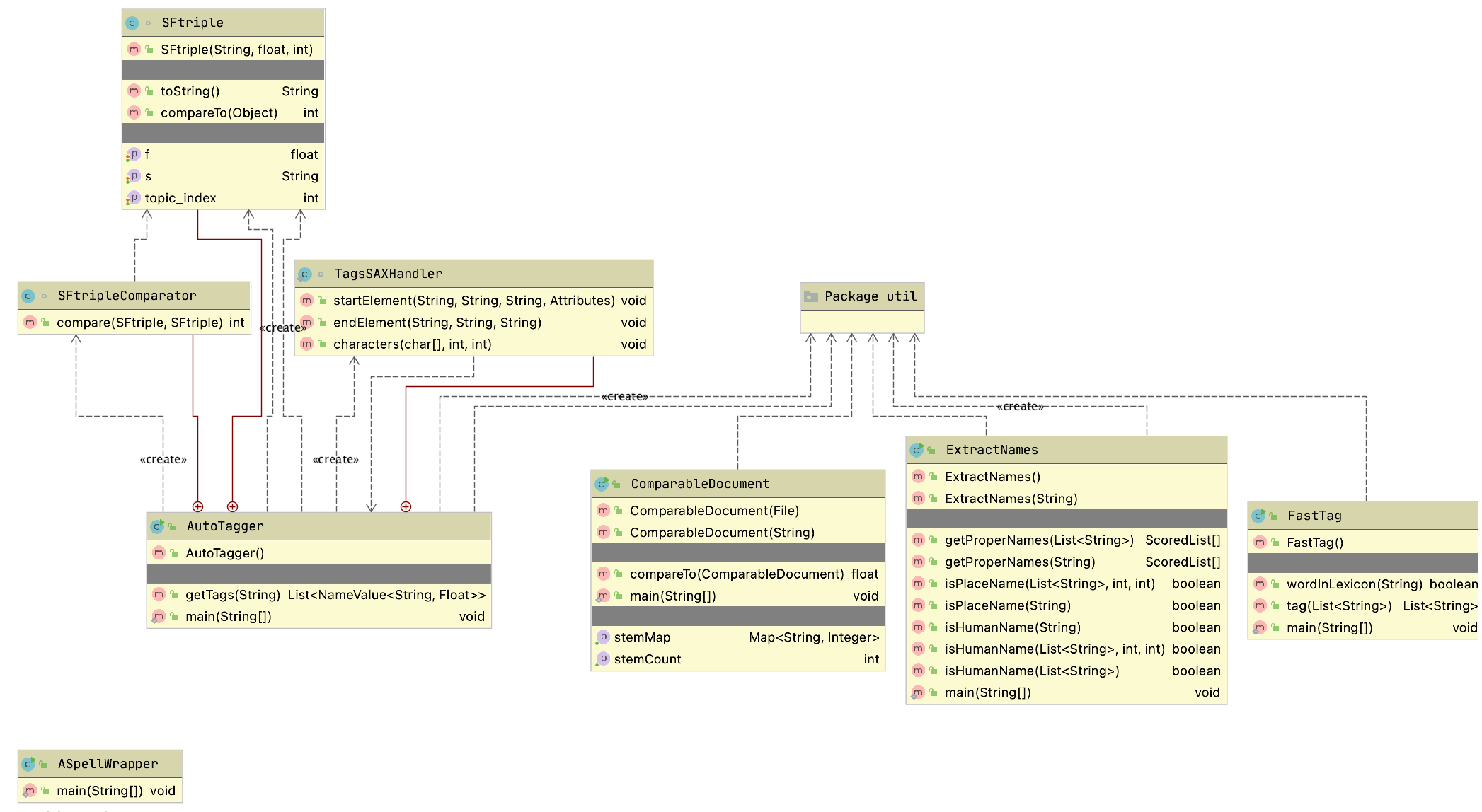
The XML parsing code is for reading the file test_data/classification_tags.xml that contains ranked word terms for various categories we cover (e.g., politics, economy, etc.), often referred to as term frequency–inverse document frequency (tf-idf).
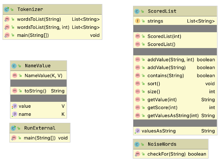
Each main class in this library has a main method that provides a short demonstration of using the class. The Makefile has targets for running the main method for each of the top level classes:
 1 names:
 2   mvn install -DskipTests
 3   mvn exec:java -Dexec.mainClass="com.markwatson.nlp.ExtractNames"
 4
 5 autotagger:
 6   mvn install -DskipTests
 7   mvn exec:java -Dexec.mainClass="com.markwatson.nlp.AutoTagger"
 8
 9 fasttag:
10   mvn install -DskipTests
11   mvn exec:java -Dexec.mainClass="com.markwatson.nlp.FastTag"
You might find it useful to run the examples before we look at the code.
Tokenizing, Stemming, and Part of Speech Tagging Text
Tokenizing text is the process of splitting a string containing text into individual tokens. Stemming is the reduction of words to abbreviated word roots that allow for easy comparison for equality of similar words. Tagging is identifying what part of speech each word is in input text. Tagging is complicated by many words having different parts of speech depending on context (examples: “bank the airplane,” “the river bank,” etc.) You can find the code in this section in the GitHub repository in the files src/com/markwatson/nlp/fasttag/FastTag.java and src/com/markwatson/nlp/util/Tokenizer.java. The required data files are in the directory test_data in the files lexicon.txt (for processing English text) and lexicon_medpost.txt (for processing medical text).
We will also look at a public domain word stemmer that I frequently use in this section.
Before we can process any text we need to break text into individual tokens. Tokens can be words, numbers and punctuation symbols. The class Tokenizer has two static methods, both take an input string to tokenize and return a list of token strings. The second method has an extra argument to specify the maximum number of tokens that you want returned:
1       static public List<String> wordsToList(String s)
2       static public List<String> wordsToList(String s, int maxR)
In line 2, maxR is maximum number of tokens to return and is useful when you want to sample the first part of a very long text.
The following listing shows a fragment of example code using this class with the output:
       String text =
         "The ball, rolling quickly, went down the hill.";
       List<String> tokens = Tokenizer.wordsToList(text);
       System.out.println(text);
       for (String token : tokens)
          System.out.print("\""+token+"\" ");
       System.out.println();
This code fragment produces the following output:
For many applications, it is better to “stem” word tokens to simplify comparison of similar words. For example “run,” “runs,” and “running” all stem to “run.” The stemmer that we will use, which I believe to be in the public domain, is in the file src/public_domain/Stemmer.java. There are two convenient APIs defined at the end of the class, one to stem a string of multiple words and one to stem a single word token:
My FastTag part of speech (POS) tagger project resulted from my using in the early 1990s the excellent tagger written by Eric Brill while he was at the University of Pennsylvania. He used machine learning techniques to learn transition rules for tagging text using manually tagged text as training examples. In reading through his doctoral thesis I noticed that there were a few transition rules that covered most of the cases and I implemented a simple “fast tagger” in Common Lisp, Ruby, Scheme and Java. The Java version is in the file src/com/markwatson/nlp/fasttag/FastTag.java.
The file src/com/markwatson/nlp/fasttag/README.txt contains information on where to obtain Eric Brill’s original tagging system and also defines the tags for both his English language lexicon and the Medpost lexicon. The following table shows the most commonly used tags (see the README.txt file for a complete description).
Brill’s system worked by processing manually tagged text and then creating a list of words followed by the tags found for each word. Here are a few random lines selected from the test_data/lexicon.txt file:
Here “Arco” is a proper noun because it is the name of a corporation. The word “Arctic” can be either a proper noun or an adjective; it is used most frequently as a proper noun so the tag “NNP” is listed before “JJ.” The word “fair” can be an adjective, singular noun, or an adverb.
The class Tagger reads the file lexicon either as a resource stream (if, for example, you put lexicon.txt **in the same JAR file as the compiled **Tagger and Tokenizer class files) or as a local file. Each line in the lexicon.txt file is passed through the utility method parseLine that processes an input string using the first token in the line as a hash key and places the remaining tokens in an array that is the hash value. So, we would process the line “fair JJ NN RB” as a hash key of “fair” and the hash value would be the array of strings (only the first value is currently used but I keep the other values for future use).
When the tagger is processing a list of word tokens, it looks each token up in the hash table and stores the first possible tag type for the word. In our example, the word “fair” would be assigned (possibly temporarily) the tag “JJ.” We now have a list of word tokens and an associated list of possible tag types. We now loop through all of the word tokens applying eight transition rules that Eric Brill’s system learned. We will look at the first rule in some detail; i is the loop variable in the range [0, number of word tokens - 1] and word is the current word at index i:
      //  rule 1: DT, {VBD | VBP} --> DT, NN
      if (i > 0 && ret.get(i - 1).equals("DT")) {
          if (word.equals("VBD") ||
              word.equals("VBP") ||
              word.equals("VB")) {
                         ret.set(i, "NN");
          }
      }
In English, this rule states that if a determiner (DT) at word token index i - 1 is followed by either a past tense verb (VBD) or a present tense verb (VBP) then replace the tag type at index i with “NN.”
I list the remaining seven rules in a short syntax here and you can look at the Java source code to see how they are implemented:
      rule 2: convert a noun to a number (CD) if "."
              appears in the word
      rule 3: convert a noun to a past participle if
              words.get(i) ends with "ed"
      rule 4: convert any type to adverb if it ends in "ly"
      rule 5: convert a common noun (NN or NNS) to an
              adjective if it ends with "al"
      rule 6: convert a noun to a verb if the preceding
              work is "would"
      rule 7: if a word has been categorized as a common
              anoun nd it ends with "s", then set its type
              to plural common noun (NNS)
      rule 8: convert a common noun to a present participle
              verb (i.e., a gerund)
My FastTag tagger is not quite as accurate as Brill’s original tagger so you might want to use his system written in C but which can be executed from Java as an external process or with a JNI interface.
In the next section we will use the tokenizer, stemmer, and tagger from this section to develop a system for identifying named entities in text.
Named Entity Extraction From Text
In this section we will look at identifying names of people and places in text. This can be useful for automatically tagging news articles with the people and place names that occur in the articles. The “secret sauce” for identifying names and places in text is the data in the file test_data/propername.ser – a serialized Java data file containing hash tables for human and place names. This data is read in the constructor for the class Names; it is worthwhile looking at the code if you have not used the Java serialization APIs before:
      ObjectInputStream p = new ObjectInputStream(ins);
      Hashtable lastNameHash = (Hashtable) p.readObject();
      Hashtable firstNameHash = (Hashtable) p.readObject();
      Hashtable placeNameHash = (Hashtable) p.readObject();
      Hashtable prefixHash = (Hashtable) p.readObject();
If you want to see these data values, use code like
      Enumeration keysE = placeNameHash.keys();
      while (keysE.hasMoreElements()) {
        Object key = keysE.nextElement();
        System.out.println(key + " : " +
                           placeNameHash.get(key));
      }
The small part of the output from running this code snippet is:
Before we look at the entity extraction code and how it works, we will first look at an example of using the main APIs for the Names class. The following example uses the methods isPlaceName, isHumanName, and getProperNames:
      System.out.println("Los Angeles: " +
                  names.isPlaceName("Los Angeles"));
      System.out.println("President Bush: " +
                  names.isHumanName("President Bush"));
      System.out.println("President George Bush: " +
           names.isHumanName("President George Bush"));
      System.out.println("President George W. Bush: " +
           names.isHumanName("President George W. Bush"));
      ScoredList[] ret = names.getProperNames(
            "George Bush played golf. President     \
             George W. Bush went to London England, \
             and Mexico to see Mary    \
             Smith in Moscow. President Bush will   \
             return home Monday.");
      System.out.println("Human names: " +
                         ret[0].getValuesAsString());
      System.out.println("Place names: " +
                         ret[1].getValuesAsString());
The output from running this example is:
The complete implementation that you can read through in the source file ExtractNames.java is reasonably simple. The methods isHumanName and isPlaceName simply look up a string in either of the human or place name hash tables. For testing a single word this is very easy; for example:
      public boolean isPlaceName(String name) {
        return placeNameHash.get(name) != null;
      }
The versions of these APIs that handle names containing multiple words are just a little more complicated; we need to construct a string from the words between the starting and ending indices and test to see if this new string value is a valid key in the human names or place names hash tables. Here is the code for finding multi-word place names:
      public boolean isPlaceName(List<String> words,
                                 int startIndex,
                                 int numWords) {
        if ((startIndex + numWords) > words.size()) {
          return false;
        }
        if (numWords == 1) {
          return isPlaceName(words.get(startIndex));
        }
        String s = "";
        for (int i=startIndex;
             i<(startIndex + numWords); i++) {
          if (i < (startIndex + numWords - 1)) {
            s = s + words.get(startIndex) + " ";
          } else {
            s = s + words.get(startIndex);
          }
        }
        return isPlaceName(s);
      }
This same scheme is used to test for multi-word human names. The top-level utility method getProperNames is used to find human and place names in text. The code in getProperNames is intentionally easy to understand but not very efficient because of all of the temporary test strings that need to be constructed.
Automatically Assigning Categories to Text
Here we will assign zero or more categories like “politics”, “economy”, etc. to text based on the words contained in the text. While the code for doing this is simple there is usually much work to do to build a word count database for different classifications. The approach we use here is often called “bag of words” because the words in input text matter but not the order of words in text or proximity to other words.
I have been working on open source products for automatic tagging and semantic extraction since the 1990s (see my old web site www.knowledgebooks.com if you are interested). In this section I will show you some simple techniques for automatically assigning tags or categories to text. We will use a set of category tags for which I have collected word frequency statistics. For example, a category of “Java” might be associated with the use of the words “Java,” “JVM,” “Sun,” etc. You can find my pre-trained tag data in the file:
The Java source code for the class AutoTagger is in the file:
The AutoTagger class uses a few data structures to keep track of both the names of categories (tags) and the word count statistics for words associated with each tag name. I use a temporary hash table for processing the XML input data:
private static Hashtable<String, Hashtable<String, Float>> tagClasses;
The names of categories (tags) used are defined in the XML tag data file: change this file, and you alter both the tags and behavior of this utility class. Please note that the data in this XML file is from a small set of hand-labeled text found on the Web (i.e., my wife and I labelled articles as being about “religion”, “politics”, etc.).
This approach is called “bag of words.” The following listing shows a snippet of data defined in the XML tag data file describing some words (and their scores) associated with the tag “religion_buddhism”:
    <tags>
      <topic name="religion_buddhism">
        <term name="buddhism" score="52" />
        <term name="buddhist" score="50" />
        <term name="mind" score="50" />
        <term name="buddha" score="37" />
        <term name="practic" score="31" />
        <term name="teach" score="15" />
        <term name="path" score="14" />
        <term name="mantra" score="14" />
        <term name="thought" score="14" />
        <term name="school" score="13" />
        <term name="zen" score="13" />
        <term name="mahayana" score="13" />
        <term name="suffer" score="12" />
        <term name="dharma" score="12" />
        <term name="tibetan" score="11" />
        . . .
      </topic>
      . . .
    </tags>
Notice that the term names are stemmed words and all lower case. There are 28 categories (tags) defined in the input XML file included in the GitHub repository for this book.
For data access, I also maintain an array of tag names and an associated list of the word frequency hash tables for each tag name:
      private static String[] tagClassNames;
      private static
        List<Hashtable<String, Float>> hashes =
           new ArrayList<Hashtable<String, Float>>();
The XML data is read and these data structures are filled during static class load time so creating multiple instances of the class AutoTagger has no performance penalty in memory use. Except for an empty default class constructor, there is only one public API for this class, the method getTags gets the categories for input text:
      public List<NameValue<String, Float>>
                     getTags(String text) {
To be clear, the tags returned are classification tags like “politics,” “economy,” etc. The utility class NameValue is defined in the file:
To determine the tags for input text, we keep a running score for each defined tag type. I use the internal class SFtriple to hold triple values of word, score, and tag index. I choose the tags with the highest scores as the automatically assigned tags for the input text. Scores for each tag are calculated by taking each word in the input text, stemming it, and if the stem is in the word frequency hash table for the tag then add the score value in the hash table to the running sum for the tag. You can refer to the AutoTagger.java source code for details. Here is an example use of class AutoTagger:
      AutoTagger test = new AutoTagger();
      String s = "The President went to Congress to argue
                  for his tax bill before leaving on a
                  vacation to Las Vegas to see some shows
                  and gamble.";
      List<NameValue<String, Float>> results =
                                        test.getTags(s);
      for (NameValue<String, Float> result : results) {
        System.out.println(result);
      }
The output looks like:
Text Clustering
Clustering text documents refers to associating similar text documents with each other. The text clustering system that I have written for my own projects is simple and effective but it inefficient for large numbers of documents. The example code in this section is inherently inefficient for clustering a large number of text documents because I perform significant semantic processing on each text document and then compare all combinations of documents. The runtime performance is O(N2) where N is the number of text documents. If you need to cluster or compare a very large number of documents you will probably want to use a K-Mean clustering algorithm instead.
I use a few different algorithms to rate the similarity of any two text documents and I will combine these depending on the requirements of the project that I am working on:
- Calculate the intersection of common words in the two documents.
- Calculate the intersection of common word stems in the two documents.
- Calculate the intersection of tags assigned to the two documents.
- Calculate the intersection of human and place names in the two documents.
In this section we will implement the second option: calculate the intersection of word stems in two documents. Without showing the package and import statements, it takes just a few lines of code to implement this algorithm when we use the Stemmer class.
The following listing shows the implementation of class ComparableDocument with comments. We start by defining constructors for documents defined by a File object and a String object:
    public class ComparableDocument {
        // disable default constructor calls:
        private ComparableDocument() { }
        public ComparableDocument(File document)
                     throws FileNotFoundException {
            this(new Scanner(document).
                       useDelimiter("\\Z").next());
        }
        public ComparableDocument(String text) {
            List<String> stems =
                   new Stemmer().stemString(text);
            for (String stem : stems) {
                stem_count++;
                if (stemCountMap.containsKey(stem)) {
                    Integer count = stemCountMap.get(stem);
                    stemCountMap.put(stem, 1 + count);
                } else {
                    stemCountMap.put(stem, 1);
                }
            }
        }
In the last constructor, I simply create a count of how many times each stem occurs in the document.
The public API allows us to get the stem count hash table, the number of stems in the original document, and a numeric comparison value for comparing this document with another (this is the first version – we will add an improvement later):
      public Map<String, Integer> getStemMap() {
        return stemCountMap;
      }
      public int getStemCount() {
        return stem_count;
      }
      public float
             compareTo(ComparableDocument otherDocument) {
        long count = 0;
        Map<String,Integer> map2 = otherDocument.getStemMap();
        Iterator iter = stemCountMap.keySet().iterator();
        while (iter.hasNext()) {
          Object key = iter.next();
          Integer count1 = stemCountMap.get(key);
          Integer count2 = map2.get(key);
          if (count1!=null && count2!=null) {
            count += count1 * count2;
          }
        }
        return (float) Math.sqrt(
                 ((float)(count*count) /
                  (double)(stem_count *
                           otherDocument.getStemCount())))
                / 2f;
      }
      private Map<String, Integer> stemCountMap =
                        new HashMap<String, Integer>();
      private int stem_count = 0;
    }
I normalize the return value for the method compareTo to return a value of 1.0 if compared documents are identical (after stemming) and 0.0 if they contain no common stems. There are four test text documents in the test_data directory and the following test code compares various combinations. Note that I am careful to test the case of comparing identical documents:
      ComparableDocument news1 =
         new ComparableDocument("testdata/news_1.txt");
      ComparableDocument news2 =
         new ComparableDocument("testdata/news_2.txt");
      ComparableDocument econ1 =
         new ComparableDocument("testdata/economy_1.txt");
      ComparableDocument econ2 =
         new ComparableDocument("testdata/economy_2.txt");
      System.out.println("news 1 - news1: " +
                         news1.compareTo(news1));
      System.out.println("news 1 - news2: " +
                         news1.compareTo(news2));
      System.out.println("news 2 - news2: " +
                         news2.compareTo(news2));
      System.out.println("news 1 - econ1: " +
                         news1.compareTo(econ1));
      System.out.println("econ 1 - econ1: " +
                         econ1.compareTo(econ1));
      System.out.println("news 1 - econ2: " +
                         news1.compareTo(econ2));
      System.out.println("econ 1 - econ2: " +
                         econ1.compareTo(econ2));
      System.out.println("econ 2 - econ2: " +
                         econ2.compareTo(econ2));
The following listing shows output that indicates mediocre results; we will soon make an improvement that makes the results better. The output for this test code is:
There is not as much differentiation in comparison scores between political news stories and economic news stories. What is up here? The problem is that I did not remove common words (and therefore common word stems) when creating stem counts for each document. I wrote a utility class NoiseWords for identifying both common words and their stems; you can see the implementation in the file NoiseWords.java. Removing noise words improves the comparison results (I added a few tests since the last printout):
Much better results! The API for com.markwatson.nlp.util.NoiseWords is a single static method:
public static boolean checkFor(String stem)
You can add additional noise words to the data section in the file NoiseWords.java, depending on your application.
Wrapup
This chapter contains my own experiments with ad-hoc NLP that I often find useful for my work.
In the next chapter Natural Language Processing Using OpenNLP we use the Apache OpenNLP library that I also often use in my work.
Natural Language Processing Using OpenNLP
Here we use the Apache OpenNLP project. OpenNLP has pre-trained models for tokenization, sentence segmentation, part-of-speech tagging, named entity extraction, chunking, parsing, and coreference resolution. As we see later OpenNLP has tools to also build our own models.
I have worked in the field of Natural Language Processing (NLP) since the early 1980s. Many more people are now interested in the field of NLP and the techniques have changed drastically in the last decade.
Currently, OpenNLP has support for Danish, German, English, Spanish, Portuguese, and Swedish. I include in the github repository some trained models for English that are used in the examples in this chapter. You can download models for other languages at the web page for OpenNLP 1.5 models (we are using version 1..6.0 of OpenNLP in this book which uses the version 1.5 models).
The following figure shows the project for this chapter in the Community Edition of IntelliJ:
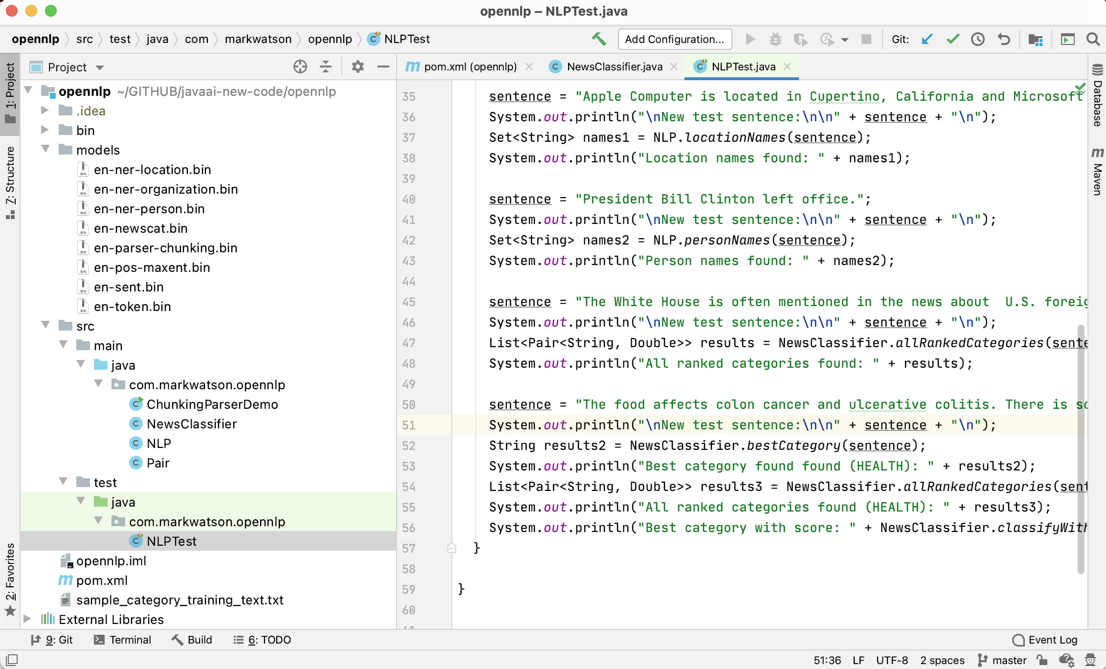
We will use pre-trained models for tokenizing text, recognizing the names of organizations, people, locations, and parts of speech for words in input text. We will also train a new model (the file opennlp/models/en-newscat.bin in the github repository) for recognizing the category of input text. The section on training new maximum entropy classification models using your own training data may be the material in this chapter that you will use the most in your own projects. We will train one model to recognize the categories of COMPUTERS, ECONOMY, HEALTH, and POLITICS. You should then have the knowledge for training your own models using your own training texts for the categories that you need for your applications. The OpenNLP documentation has additional detail on custom models. We will also use both some pre-trained models that are included with the OpenNLP distribution in the next chapter when we combine using OpenNLP with the WordNet lexical database developed at Princeton University.
After building a classification model we finish up this chapter with an interesting topic: statistically parsing sentences to discover the most probable linguistic structure of each sentence in input text. We will not use parsing in the rest of this book so you may skip the last section of this chapter if you are not currently interested in understanding sentence parse tree structure of components like noun and verb phrases, proper nouns, nouns, and adjectives, etc.
The following UML class diagrams will give you an overview of my wrapper for the OpenNLP library and for the unit test class:
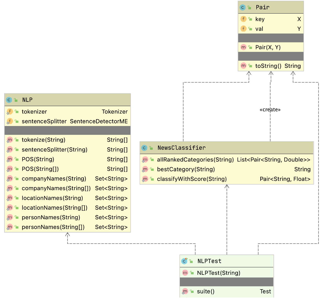
Using OpenNLP Pre-Trained Models
Assuming that you have cloned the github repository for this book, you can fetch the maven dependencies, compile the code, install the generated library locally, and run the unit tests using the command:
The model files, including the categorization model you will learn to build later in this chapter, are found in the subdirectory models. The unit tests in src/test/java/com/markwatson/opennlp/NLPTest.java provide examples for using the code we develop in this chapter. As for many examples in this book, I use unit tests as examples for using a library and not as tests that check computed values.
The Java example code for tokenization (splitting text into individual words), splitting sentences, and recognizing organizations, locations, and people in text is all in the Java class NLP. You can look at the source code in the repository for this book. Here I will just show a few snippets of the code to make clear how to load and use pre-trained models.
I use static class initialization to load the model files:
  static public Tokenizer tokenizer = null;
  static public SentenceDetectorME sentenceSplitter = null;
  static POSTaggerME tagger = null;
  static NameFinderME organizationFinder = null;
  static NameFinderME locationFinder = null;
  static NameFinderME personNameFinder = null;

  static {

    try {
      InputStream organizationInputStream =
	    new FileInputStream("models/en-ner-organization.bin");
      TokenNameFinderModel model =
	    new TokenNameFinderModel(organizationInputStream);
      organizationFinder = new NameFinderME(model);
      organizationInputStream.close();

      InputStream locationInputStream =
	    new FileInputStream("models/en-ner-location.bin");
      model = new TokenNameFinderModel(locationInputStream);
      locationFinder = new NameFinderME(model);
      locationInputStream.close();

      InputStream personNameInputStream =
	    new FileInputStream("models/en-ner-person.bin");
      model = new TokenNameFinderModel(personNameInputStream);
      personNameFinder = new NameFinderME(model);
      personNameInputStream.close();

      InputStream tokienizerInputStream =
	    new FileInputStream("models/en-token.bin");
      TokenizerModel modelTokenizer = new TokenizerModel(tokienizerInputStream);
      tokenizer = new TokenizerME(modelTokenizer);
      tokienizerInputStream.close();

      InputStream sentenceInputStream =
	    new FileInputStream("models/en-sent.bin");
      SentenceModel sentenceTokenizer = new SentenceModel(sentenceInputStream);
      sentenceSplitter = new SentenceDetectorME(sentenceTokenizer);
      tokienizerInputStream.close();

      organizationInputStream = new FileInputStream("models/en-pos-maxent.bin");
      POSModel posModel = new POSModel(organizationInputStream);
      tagger = new POSTaggerME(posModel);

    } catch (IOException e) {
      e.printStackTrace();
    }
  }
The first operation that you will usually start with for processing natural language text is breaking input text into individual words and sentences. Here is the code for using the tokenizing code that separates text stored as a Java String into individual words:
  public static String[] tokenize(String s) {
    return tokenizer.tokenize(s);
  }
Here is the similar code for breaking text into individual sentences:
  public static String[] sentenceSplitter(String s) {
    return sentenceSplitter.sentDetect(s);
  }
Here is some sample code to use sentenceSplitter:
1     String sentence =
2       "Apple Computer, Microsoft, and Google are in the " +
3       " tech sector. Each is very profitable.";
4     String [] sentences = NLP.sentenceSplitter(sentence);
5     System.out.println("Sentences found:\n" + Arrays.toString(sentences));
In line 4 the static method NLP.sentenceSplitter returns an array of strings. In line 5 I use a common Java idiom for printing arrays by using the static method Arrays.toString to convert the array of strings into a List<String> object. The trick is that the List class has a toString method that formats list nicely for printing.
Here is the output of this code snippet (edited for page width and clarity):
The code for finding organizations, locations, and people’s names is almost identical so I will only show the code in the next listing for recognizing locations. Please look at the methods companyNames and personNames in the class com.markwatson.opennlp.NLP to see the implementations for finding the names of companies and people.
 1   public static Set<String> locationNames(String text) {
 2     return locationNames(tokenizer.tokenize(text));
 3   }
 4
 5   public static Set<String> locationNames(String tokens[]) {
 6     Set<String> ret = new HashSet<String>();
 7     Span[] nameSpans = locationFinder.find(tokens);
 8     if (nameSpans.length == 0) return ret;
 9     for (int i = 0; i < nameSpans.length; i++) {
10       Span span = nameSpans[i];
11       StringBuilder sb = new StringBuilder();
12       for (int j = span.getStart(); j < span.getEnd(); j++)
13         sb.append(tokens[j] + " ");
14       ret.add(sb.toString().trim().replaceAll(" ,", ","));
15     }
16     return ret;
17   }
The public methods in the class com.markwatson.opennlp.NLP are overriden to take either a single string value which gets tokenized inside of the method and also a method that takes as input text that has already been tokenized into a String tokens[] object. In the last example the method starting on line 1 accepts an input string and the overriden method starting on line 5 accepts an array of strings. Often you will want to tokenize text stored in a single input string into tokens and reuse the tokens for calling several of the public methods in com.markwatson.opennlp.NLP that can take input that is already tokenized. In line 2 we simply tokenize the input text and call the method that accepts tokenized input text.
In line 6 we create a HashSet<String> object that will hold the return value of a set of location names. The NameFinderME object locationFinder returns an array of Span objects. The Span class is used to represent a sequence of adjacent words. The Span class has a public static attribute length and instance methods getstart and getEnd that return the indices of the beginning and ending (plus one) index of a span in the original input text.
Here is some sample code to use locationNames along with the output (edited for page width and clarity):
   String sentence =
     "Apple Computer is located in Cupertino, California and Microsoft " +
     "is located in Seattle, Washington. He went to Oregon";
   Set<String> names = NLP.locationNames(sentence);
   System.out.println("Location names found: " + names);
Location names found: [Oregon, Cupertino, Seattle, California, Washington]
Note that the pre-trained model does not provide information when city and state names are associated with each other in the original sentence. The maximum entropy models used in OpenNLP do use information on the context or a word in a sentence, for example, the preceeding and following word. This combination of available contextual information makes maximum entropy models more accurate than the “bag of words” technique we used in the last chapter.
Training a New Categorization Model for OpenNLP
The OpenNLP class DoccatTrainer can process specially formatted input text files and produce categorization models using maximum entropy which is a technique that handles data with many features. Features that are automatically extracted from text and used in a model are things like words in a document and word adjacency. Maximum entropy models can recognize multiple classes. In testing a model on new text data the probablilities of all possible classes add up to the value 1 (this is often refered to as “softmax”). For example we will be training a classifier on four categories and the probablilities of these categories for some test input text add up to the value of one:
The format of the input file for training a maximum entropy classifier is simple but has to be correct: each line starts with a category name, followed by sample text for each category which must be all on one line. Please note that I have already trained the model producing the model file models/en-newscat.bin so you don’t need to run the example in this section unless you want to regenerate this model file.
The file sample_category_training_text.txt contains four lines, defining four categories. Here are two lines from this file (I edited the following to look better on the printed page, but these are just two lines in the file):
Here is one training example each for the categories COMPUTERS and ECONOMY.
You must format the training file perfectly. As an example, if you have empty (or blank) lines in your input training file then you will get an error like:
The OpenNLP documentation has examples for writing custom Java code to build models but I usually just use the command line tool; for example:
The model is written to the relative file path models/en-newscat.bin. The training file I am using is tiny so the model is trained in a few seconds. For serious applications, the more training text the better! By default the DoccatTrainer tool uses the default text feature generator which uses word frequencies in documents but ignores word ordering. As I mention in the next section, I sometimes like to mix word frequency feature generation with 2gram (that is, frequencies of two adjacent words). In this case you cannot simply use the DoccatTrainer command line tool. You need to write a little Java code yourself that you can plug another feature generator into using the alternative API:
public static DoccatModel train(String languageCode,
                                ObjectStream<DocumentSample> samples,
                                int cutoff, int iterations,
                                FeatureGenerator... featureGenerators)
In the next section, you will note that the last argument would look like the case where we combine two feature generators, one that uses “bag of words” and the other that uses adjacent word sequences:
public DocumentCategorizerME(DoccatModel model,
           new FeatureGenerator[]{new BagOfWordsFeatureGenerator(),
                                  new NGramFeatureGenerator()});
For some purposes the default word frequency (or bag of words) feature generator is probably OK so using the command line tool is a good place to start because models are smaller and training time is minimal. Adding the NGramFeatureGenerator increases both training time and model size but should produce better results. Here is the output from running the DoccatTrainer command line tool:
> bin/opennlp DoccatTrainer -model models/en-newscat.bin -lang en \
                            -data sample_category_training_text.txt \
                            -encoding UTF-8
Indexing events using cutoff of 5

	Computing event counts...  done. 4 events
	Indexing...  done.
Sorting and merging events... done. Reduced 4 events to 4.
Done indexing.
Incorporating indexed data for training...
done.
	Number of Event Tokens: 4
	    Number of Outcomes: 4
	  Number of Predicates: 153
...done.
Computing model parameters ...
Performing 100 iterations.
  1:  ... loglikelihood=-5.545177444479562	0.25
  2:  ... loglikelihood=-4.730232204542369	0.5
  3:  ... loglikelihood=-4.232192673282495	0.75
   ...
 98:  ... loglikelihood=-0.23411803835475453	1.0
 99:  ... loglikelihood=-0.23150121909902377	1.0
100:  ... loglikelihood=-0.22894028845170055	1.0
Writing document categorizer model ... done (0.041s)

Wrote document categorizer model to
path: /Users/mark/power-java/opennlp/models/en-newscat.bin
We will use our new trained model file en-newscat.bin in the next section.
Please note that in this simple example I used very little data, just a few hundred words for each training category. I have used the OpenNLP maximum entropy library on various projects, mostly to good effect, but I used many thousands of words for each category. The more data, the better.
Using Our New Trained Classification Model
The code that uses the model we trained in the last section is short enough to list in its entirety:
 1 package com.markwatson.opennlp;
 2
 3 import opennlp.tools.doccat.DoccatModel;
 4 import opennlp.tools.doccat.DocumentCategorizerME;
 5
 6 import java.io.*;
 7 import java.util.*;
 8
 9 /**
10  * This program uses the maximum entropy model we trained
11  * using the instructions in the chapter on OpenNLP in the book.
12  */
13
14 public class NewsClassifier {
15
16   public static List<Pair<String,Double>> allRankedCategories(String text) {
17     DocumentCategorizerME aCategorizer = new DocumentCategorizerME(docCatModel);
18     double[] outcomes = aCategorizer.categorize(text);
19     List<Pair<String,Double>> results = new ArrayList<Pair<String, Double>>();
20     for (int i=0; i<outcomes.length; i++) {
21       results.add(new Pair<String, Double>(aCategorizer.getCategory(i), outcomes[i])\
22 );
23     }
24     return results;
25   }
26
27   public static String bestCategory(String text) {
28     DocumentCategorizerME aCategorizer = new DocumentCategorizerME(docCatModel);
29     double[] outcomes = aCategorizer.categorize(text);
30     return aCategorizer.getBestCategory(outcomes);
31   }
32
33   public static Pair<String,Float> classifyWithScore(String text) {
34     DocumentCategorizerME classifier = new DocumentCategorizerME(docCatModel);
35     double [] scores = classifier.categorize(text);
36     int num_categories = classifier.getNumberOfCategories();
37     if (num_categories > 0) {
38       String bestString =  classifier.getBestCategory(scores);
39       for (int i=0; i<num_categories; i++) {
40         if (classifier.getCategory(i).equals(bestString)) {
41           return new Pair<String,Float>(bestString, (float)scores[i]);
42         }
43       }
44     }
45     return new Pair<String,Float>("<no category>", 0f);
46   }
47
48   static DoccatModel docCatModel = null;
49
50   static {
51
52     try {
53       InputStream modelIn = new FileInputStream("models/en-newscat.bin");
54       docCatModel = new DoccatModel(modelIn);
55     } catch (IOException e) {
56       e.printStackTrace();
57     }
58   }
59 }
In lines 48-57 we initialize the static data for an instance of the class DoccatModel that loads the model file created in the last section.
A new instance of the class DocumentCategorizerME is created in line 28 each time we want to classify input text. I called the one argument constructor for this class that uses the default feature detector. An alternative constructor is:
public DocumentCategorizerME(DoccatModel model,
                             FeatureGenerator... featureGenerators)
The default feature generator is BagOfWordsFeatureGenerator which just uses word frequencies for classification. This is reasonable for smaller training sets as we used in the last section but when I have a large amount of training data available I prefer to combine BagOfWordsFeatureGenerator with NGramFeatureGenerator. You would use the constructor call:
public DocumentCategorizerME(DoccatModel model,
           new FeatureGenerator[]{new BagOfWordsFeatureGenerator(),
                                  new NGramFeatureGenerator()});
The following listings show interspersed both example code snippets for using the NewsClassifier class followed by the output printed by each code snippet:
    String sentence = "Apple Computer, Microsoft, and Google are in the tech sector.\
 Each is very profitable.";
    System.out.println("\nNew test sentence:\n\n" + sentence + "\n");
    String [] sentences = NLP.sentenceSplitter(sentence);
    System.out.println("Sentences found: " + Arrays.toString(sentences));

New test sentence:

Apple Computer, Microsoft, and Google are in the tech sector.
Each is very profitable.

Sentences found: [Apple Computer, Microsoft, and Google are in the tech sector.,
                  Each is very profitable.]
    sentence = "Apple Computer, Microsoft, and Google are in the tech sector.";
    Set<String> names = NLP.companyNames(sentence);
    System.out.println("Company names found: " + names);

Company names found: [Apple Computer, Microsoft]

    sentence = "Apple Computer is located in Cupertino, California and Microsoft is \
located in Seattle, Washington. He went to Oregon";
    System.out.println("\nNew test sentence:\n\n" + sentence + "\n");
    Set<String> names1 = NLP.locationNames(sentence);
    System.out.println("Location names found: " + names1);

New test sentence:

Apple Computer is located in Cupertino, California and Microsoft is located in Seatt\
le, Washington. He went to Oregon

Location names found: [Oregon, Cupertino, Seattle, California, Washington]
    sentence = "President Bill Clinton left office.";
    System.out.println("\nNew test sentence:\n\n" + sentence + "\n");
    Set<String> names2 = NLP.personNames(sentence);
    System.out.println("Person names found: " + names2);

New test sentence:

President Bill Clinton left office.

Person names found: [Bill Clinton]

    sentence = "The White House is often mentioned in the news about U.S. foreign po\
licy. Members of Congress and the President are worried about the next election and \
may pander to voters by promising tax breaks. Diplomacy with Iran, Iraq, and North K\
orea is non existent in spite of a worry about nuclear weapons. A uni-polar world re\
fers to the hegemony of one country, often a militaristic empire. War started with a\
 single military strike. The voting public wants peace not war. Democrats and Republ\
icans argue about policy.";
    System.out.println("\nNew test sentence:\n\n" + sentence + "\n");
    List<Pair<String, Double>> results = NewsClassifier.allRankedCategories(sentence\
);
    System.out.println("All ranked categories found: " + results);

New test sentence:

The White House is often mentioned in the news about  U.S. foreign policy. Members o\
f Congress and the President are worried about the next election and may pander to v\
oters by promising tax breaks. Diplomacy with Iran, Iraq, and North Korea is non exi\
stent in spite of a worry about nuclear weapons. A uni-polar world refers to the heg\
emony of one country, often a militaristic empire. War started with a single militar\
y strike. The voting public wants peace not war. Democrats and Republicans argue abo\
ut policy.

All ranked categories found: [[COMPUTERS, 0.07257665117660535], [ECONOMY, 0.23559821\
969425127], [HEALTH, 0.29907267186308945], [POLITICS, 0.39275245726605396]]
    sentence = "The food affects colon cancer and ulcerative colitis. There is some \
evidence that sex helps keep us healthy. Eating antioxidant rich foods may prevent d\
esease. Smoking may raise estrogen levels in men and lead to heart failure.";
    System.out.println("\nNew test sentence:\n\n" + sentence + "\n");
    String results2 = NewsClassifier.bestCategory(sentence);
    System.out.println("Best category found found (HEALTH): " + results2);
    List<Pair<String, Double>> results3 = NewsClassifier.allRankedCategories(sentenc\
e);
    System.out.println("All ranked categories found (HEALTH): " + results3);
    System.out.println("Best category with score: " + NewsClassifier.classifyWithSco\
re(sentence));

New test sentence:

The food affects colon cancer and ulcerative colitis. There is some evidence that se\
x helps keep us healthy. Eating antioxidant rich foods may prevent desease. Smoking \
may raise estrogen levels in men and lead to heart failure.

Best category found found (HEALTH): HEALTH
All ranked categories found (HEALTH): [[COMPUTERS, 0.1578880260493374], [ECONOMY, 0.\
2163099374638936], [HEALTH, 0.35546925520388845], [POLITICS, 0.27033278128288035]]
Best category with score: [HEALTH, 0.35546926]
As this example shows it is simple to train new classifier models once you have prepared training data. In my work I have often needed to train models customized for specific topics.
Using the OpenNLP Parsing Model
We will use the parsing model that is included in the OpenNLP distribution to parse English language input text into syntax trees. You are unlikely to use a statistical parsing model in your work but I think you will enjoy the material in the section.
The following example code listing is long (68 lines) but I will explain the interesting parts after the listing:
 1 package com.markwatson.opennlp;
 2
 3 import opennlp.tools.cmdline.parser.ParserTool;
 4 import opennlp.tools.parser.Parse;
 5 import opennlp.tools.parser.ParserModel;
 6 import opennlp.tools.parser.chunking.Parser;
 7
 8 import java.io.FileInputStream;
 9 import java.io.IOException;
10 import java.io.InputStream;
11
12 /**
13  * Experiments with the chunking parser model
14  */
15 public class ChunkingParserDemo {
16   public Parse[] parse(String text) {
17     Parser parser = new Parser(parserModel);
18     return ParserTool.parseLine(text, parser, 5);
19   }
20
21   public void prettyPrint(Parse p) {
22     StringBuffer sb = new StringBuffer();
23     p.show(sb);
24     String s = sb.toString() + " ";
25     int depth = 0;
26     for (int i = 0, size = s.length() - 1; i < size; i++) {
27       if (s.charAt(i) == ' ' && s.charAt(i + 1) == '(') {
28         System.out.print("\n");
29         for (int j = 0; j < depth; j++) System.out.print("  ");
30       } else if (s.charAt(i) == '(') System.out.print(s.charAt(i));
31       else if (s.charAt(i) != ')' || s.charAt(i + 1) == ')')
32         System.out.print(s.charAt(i));
33       else {
34         System.out.print(s.charAt(i));
35         for (int j = 0; j < depth; j++) System.out.print("  ");
36       }
37       if (s.charAt(i) == '(') depth++;
38       if (s.charAt(i) == ')') depth--;
39     }
40     System.out.println();
41   }
42
43   static ParserModel parserModel = null;
44
45   static {
46
47     try {
48       InputStream modelIn = new FileInputStream("models/en-parser-chunking.bin");
49       parserModel = new ParserModel(modelIn);
50     } catch (IOException e) {
51       e.printStackTrace();
52     }
53   }
54
55   public static void main(String[] args) {
56     ChunkingParserDemo cpd = new ChunkingParserDemo();
57     Parse[] possibleParses =
58       cpd.parse("John Smith went to the store on his way home from work ");
59     for (Parse p : possibleParses) {
60       System.out.println("parse:\n");
61       p.show();
62       //p.showCodeTree();
63       System.out.println("\npretty printed parse:\n");
64       cpd.prettyPrint(p);
65       System.out.println("\n");
66     }
67   }
68 }
The OpenNLP parsing model is read from a file in lines 45 through 53. The static variable parserModel (instance of class ParserModel) if created in line 49 and used in lines 17 and 18 to parse input text. It is instructive to look at the intermediate calculation results. The value for variable parser defined in line 17 has a value of:
Note that the parser returned 5 different results because we specified this number in line 18. For a long sentence the parser generates a very large number of possible parses for the sentence and returns, in order of probability of being correct, the number of results we requested.
The OpenNLP chunking parser code prints out results in a flat list, one result on a line. This is difficult to read which is why I wrote the method prettyPrint (lines 21 through 41) to print the parse results indented. Here is the output from the last code example (the first parse shown is all on one line but line wraps in the following listing):
In the 1980s I spent much time on syntax level parsing. I no longer find these models very relevant to my own work.
OpenNLP is a good resource for Java programmers and its Apache 2 license is “business friendly.” If you can use software with a GPL license then please also look at the Stanford NLP libraries.
Combining the WordNet Linguistic Database With OpenNLP
Here we build on the material from the last chapter by using OpenNLP to process input text to identify parts of speech and then looking up words with their parts of speech in WordNet. You can use WordNet to look up all uses of a word so using OpenNLP as we do here is not required but I think makes a good example of blending libraries.
The WordNet linguistic database is complex and you may want to review the WordNet documentation after working through the following example of finding synonyms and hypernyms for nouns in text input.
Using the WordNet Linguistic Database
The Maven pom.xml file (that we will look at later) for this example is configured to download both the WordNet data and the extjwnl library. The home page for the WordNet project is http://wordnet.princeton.edu.
Tutorial on WordNet
The WordNet lexical database is an ongoing research project spanning decades that includes many years of effort by professional linguists. My own use of WordNet over the last twenty years has been simple, mainly using the database to determine synonyms (called synsets in WordNet) and looking at the possible parts of speech of words. For reference from a Wikipedia article on WordNet, here is a small subset of the type of relationships contained in WordNet for nouns (we will look at relations for verbs, adjectives, and adverbs at the end of this chapter):
hypernyms
:   parent is a hypernym of mother since every mother is of type parent

hyponyms
:   father (less general) is a hyponym of parent (more general)

holonym
:   building is a holonym of window because a window is part of a
    building

meronym
:   window is a meronym of building because a window is part of a
    building
I find the WordNet book (WordNet: An Electronic Lexical Database (Language, Speech, and Communication) by Christiane Fellbaum, 1998) to be a detailed reference for WordNet but there have been several new releases of WordNet since the book was published. The WordNet site and the Wikipedia article on WordNet are also good sources of information if you decide to make WordNet part of your toolkit.
When you look up words in WordNet you can optionally specify one of the following parts of speech (POS):
    POS.NOUN
    POS.VERB
    POS.ADJECTIVE
    POS.ADVERB
Rather than using Open NLP in this example to find nouns, we could try all four possible parts of speech on every input word. I was motivated to use OpenNLP partly because I wanted to provide an example of reusing a library developed in a different chapter, in this case the previous chapter on OpenNLP.
What are hypernyms? A hypernym is in a semantic type-of relationship with another word that is more general. As an example, the word “country” is a hypernym of the word “Mexico.” The opposite of hypernym is a hyponym, that is a hyponym has a more narrow meaning. The word “country” is a hyponym of the word “Mexico.”
The following example is simple. We only look up WordNet hypernyms and synonyms entries for nouns and for nouns. In the chapter wrap-up I will give you some ideas for more extended projects that you may want to do using WordNet.
Before diving into the code I want to show you what the generated synonym and hypernym data looks like.
The following two figures show the generated structured output data in a IntelliJ Community Edition debug session, in particular look at the structure of synonymMap. While I rarely use the debugger to actually debug code, I frequently us it to inspect data.
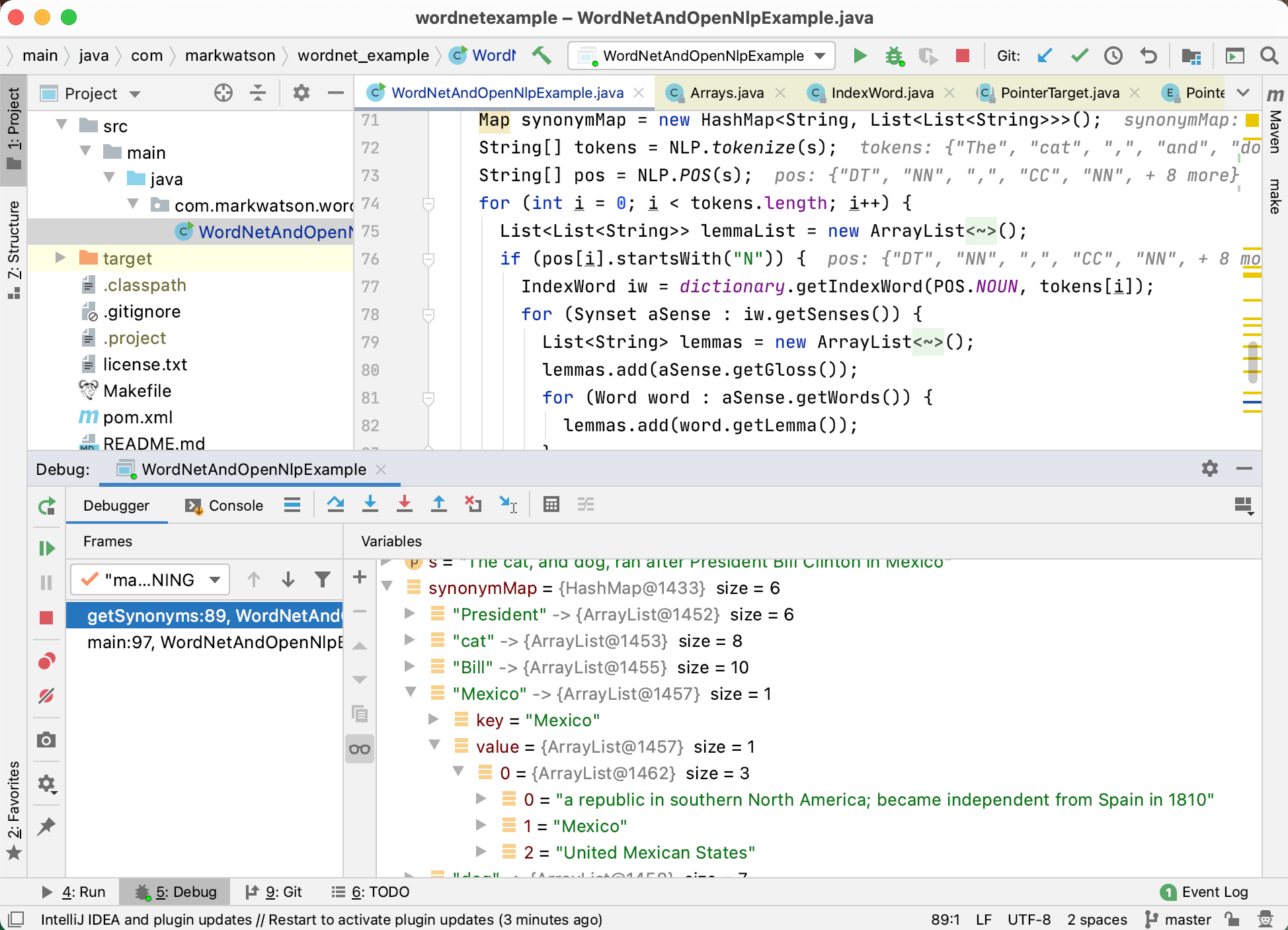
Here is a closeup showing generated data in the variable hypernymMap:
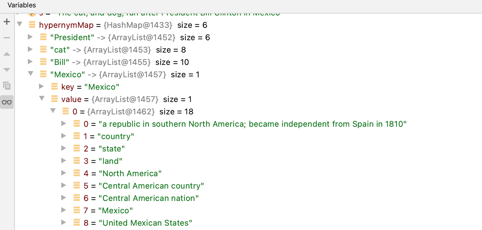
Installing the Libraries and Linguistic Data for this Example
The maven pom.xml configuration file for this project contains the following requirements:
        <dependency>
            <groupId>net.sf.extjwnl</groupId>
            <artifactId>extjwnl</artifactId>
            <version>2.0.2</version>
        </dependency>
        <!-- Princeton WordNet 3.1 data dependency -->
        <dependency>
            <groupId>net.sf.extjwnl</groupId>
            <artifactId>extjwnl-data-wn31</artifactId>
            <version>1.2</version>
        </dependency>
The second dependency loads the WordNet linguistic database.
I assume that you have performed a maven install for the project in the last chapter:
We also need the OpenNLP library and my OpenNLP wrapper library developed in the last chapter:
        <dependency>
            <groupId>opennlp</groupId>
            <artifactId>tools</artifactId>
            <version>1.5.0</version>
        </dependency>
        <dependency>
            <groupId>com.markwatson</groupId>
            <artifactId>opennlp</artifactId>
            <version>1.0-SNAPSHOT</version>
        </dependency>
There is a Makefile for running the example:
example:
 mvn install
 mvn exec:java  \
    -Dexec.mainClass="com.markwatson.wordnet_example.WordNetAndOpenNlpExample"
Run the example using:
The example identifies all nouns (in the example code they are: President, cat, Bill, Mexico, dog, and Clinton) and for each noun finds all WordNet “word senses.” The noun “Mexico” only has one word sense while the noun “cat” has eight word senses.
For each word sense (for each noun) the example code returns a list of strings where the first element is a descriptive “word gloss” for the particular sense and the remaining strings are hypernyms or synonyms depending whether we are calling the functions getHypernyms or getSynonyms whose method signatures are:
static public Map<String, List<List<String>>> getHypernyms(String s)
              throws JWNLException {
static public Map<String, List<List<String>>> getSynonyms(String s)
              throws JWNLException {
The following UML class diagram shows this public API for the example code. There is only one source file in this example WordNetAndOpenNlpExample.java because our goal here is not building a reusable library, rather to provide a short example and a “starter project” for your own experiments. That said this project does get installed as a local Maven library so you can require the library and call getHypernyms and getSynonyms in other projects. I will later suggest further projects in the wrap-up.
The values returned from both getHypernyms and getSynonyms are maps where the keys are nouns in the input text. The map value for each key (a noun) will be a list, one element for each word sense for the noun. Each of these sub-lists is a list of strings where the first element is the gloss for the word sense and the remaining strings are either hypernyms or synonyms depending of which function is called.
Let’s look at the word “Clinton” which has four different word senses; here we list the gloss for each word sense:
- wife of President Clinton and later a woman member of the United States Senate (1947-)
- 42nd President of the United States (1946-)
- United States politician who as governor of New York supported the project to build the Erie Canal (1769-1828)
- a town in east central Iowa
As an example, the hypernyms for the first word sense are: legislator, state senator, Clinton, Hiliary Clinton, etc.
WordNet is a linguistic database for automating the processing of text and does contain some “real world” knowledge but does not have the wide coverage of semantic web knowledge graphs like DBPedia and WikiData. We will discuss the semantic web and Knowledge Graphs in later chapters as a source of information. Here we seek ways to understand words in text.
Here is a small segment of the output of the example program:
**** Hypernyms:
{President=[[an executive officer of a firm or corporation, executive, executive dir\
ector, chairman of the board, chief executive officer, CEO, chief operating officer,\
chief financial officer, CFO, insider, president],
...
**** Synonyms:
{President=[[an executive officer of a firm or corporation, president], [the person \
who holds the office of head of state of the United States government; "the Presiden\t likes to jog every morning", President of the United States, United States Preside\
nt, President, Chief Executive], [the chief executive of a republic, president],
...
Implementation
You will never need to instantiate an instance of the class WordNetAndOpenNlpExample because all data is static class data and the two public methods are both static. The methods getHypernyms (lines 27-58) and getSynonyms (lines 60-81) are similar except the APIs for getting synonyms (lines 68-69) differ than those for getting hypernyms (lines 39-43). These two methods could be combined into a single method with an argument to control which APIs to use but I thought the code looked simpler as it is.
 1 package com.markwatson.wordnet_example;
 2
 3 import com.markwatson.opennlp.NLP;
 4
 5 import net.sf.extjwnl.JWNLException;
 6 import net.sf.extjwnl.data.*;
 7 import net.sf.extjwnl.data.list.PointerTargetNode;
 8 import net.sf.extjwnl.dictionary.Dictionary;
 9
10 import java.util.*;
11
12 public class WordNetAndOpenNlpExample {
13
14   private WordNetAndOpenNlpExample() {
15   }
16
17   static Dictionary dictionary = null;
18   static {
19     try {
20       dictionary = Dictionary.getDefaultResourceInstance();
21     } catch (JWNLException e) {
22       e.printStackTrace();
23       System.exit(1);
24     }
25   }
26
27   static public Map<String, List<List<String>>> getHypernyms(String s)
28       throws JWNLException {
29     Map hypernymMap = new HashMap<String, List<List<String>>>();
30     String[] tokens = NLP.tokenize(s);
31     String[] pos = NLP.POS(s);
32     for (int i = 0; i < tokens.length; i++) {
33       if (pos[i].startsWith("N")) {
34         IndexWord iw = dictionary.getIndexWord(POS.NOUN, tokens[i]);
35         List hypernymList = new ArrayList<List<List<String>>>();
36         for (Synset aSense : iw.getSenses()) {
37           List lemmaList = new ArrayList<List<String>>();
38           lemmaList.add(aSense.getGloss());
39           for (PointerTargetNode ptn : PointerUtils.getDirectHypernyms(aSense)) {
40             List<PointerTarget> pthTargets = ptn.getPointerTarget().getTargets();
41             for (Object pt : pthTargets) {
42               try {
43                 Synset spt = (Synset) pt;
44                 List<Word> words = spt.getWords();
45                 for (Word word : words) {
46                   lemmaList.add(word.getLemma());
47                 }
48               } catch (Exception ignore) {
49               }
50             }
51           }
52           hypernymList.add(lemmaList);
53         }
54         if (hypernymList.size() > 0) hypernymMap.put(tokens[i], hypernymList);
55       }
56     }
57     return hypernymMap;
58   }
59
60   static public Map<String, List<List<String>>> getSynonyms(String s)
61       throws JWNLException {
62     Map synonymMap = new HashMap<String, List<List<String>>>();
63     String[] tokens = NLP.tokenize(s);
64     String[] pos = NLP.POS(s);
65     for (int i = 0; i < tokens.length; i++) {
66       if (pos[i].startsWith("N")) {
67         List<List<String>> lemmaList = new ArrayList<List<String>>();
68         IndexWord iw = dictionary.getIndexWord(POS.NOUN, tokens[i]);
69         for (Synset aSense : iw.getSenses()) {
70           List<String> lemmas = new ArrayList<String>();
71           lemmas.add(aSense.getGloss());
72           for (Word word : aSense.getWords()) {
73             lemmas.add(word.getLemma());
74           }
75           lemmaList.add(lemmas);
76         }
77         if (lemmaList.size() > 0) synonymMap.put(tokens[i], lemmaList);
78       }
79     }
80     return synonymMap;
81   }
82
83   public static void main(String[] args)
84       throws JWNLException {
85     String s = "The cat, and dog, ran after President Bill Clinton in Mexico";
86     System.out.println("\n**** Hypernyms:\n");
87     System.out.println(getHypernyms(s));
88     System.out.println("\n**** Synonyms:\n");
89     System.out.println(getSynonyms(s));
90   }
91 }
The Java class PointerTargetNode (line 39) contains two instance variables: a Sysnset and a pointer type (e.g., noun or verb). The class Synset contains a part of speech (e.g., a noun), pointers to related synsets, descriptive words (or lemmas) for the synset, and a descriptive gloss that we have seen examples of. The class IndexWord contains a part of speech for the current word sense, a descriptive word (lemma) and a list of available synsets.
Earlier you saw two screen shots examining the output data in a IntelliJ Community Edition debug session. To better understand the Java interface to WordNet, I suggest also setting breakpoints to examine the data structures used by the net.sf.extjwnl library, especially the Java classes net.sf.extjwnl.data and net.sf.extjwnl.data.IndexWord.
Other Type Relationships Supported by WordNet
For reference (from the Wikipedia article on WordNet), here is a small subset of the type of relationships contained in WordNet for verbs shown by examples (also from the Wikipedia article):
- hypernym: travel (less general) is an hypernym of movement (more general)
- entailment: to sleep is entailed by to snore because you must be asleep to snore
Here are a few of the relations supported for nouns:
- hypernyms: canine is a hypernym of dog since every dog is of type canine
- hyponyms: dog (less general) is a hyponym of canine (more general)
- holonym : building is a holonym of window because a window is part of a building
- meronym: window is a meronym of building because a window is part of a building
Some of the related information maintained for adjectives is:
- related nouns:
- similar to
As mentioned before, I find the book WordNet: An Electronic Lexical Database (Language, Speech, and Communication) useful as is the WordNet site and the Wikipedia article on WordNet. I hope that I have motivated you, dear reader, to make WordNet and OpenNLP parts of your toolkit.
Wrap-up and Ideas for Using WordNet
WordNet provides a rich linguistic database for human linguists but although I have been using WordNet since 1999, I do not often use it in automated systems. I tend to use it for manual reference and sometimes for simple tasks like augmenting a list of terms with synonyms.
The following three sub-sections are suggested projects.
Process all possible word senses
We only used WordNet entries for nouns. You might want to make copies of the file WordNetAndOpenNlpExample.java and instead of looking up entries for nouns, you might want to try other parts of speech: verbs, adjectives, and adverbs. You might also make a copy of WordNetAndOpenNlpExample.java and don’t use OpenNLP to tag text but rather look up all four supported parts of speech for each word in the input text.
WordNet is a powerful tool for automating natural language processing but it is not easy to work with. I hope that with this simple example you are now motivated to dive in deeper and consider using WordNet for your projects, where it is appropriate to do so.
Using a Part of Speech Tagger to Use the Correct WordNet Synonyms
WordNet will give us both synonyms and antonyms (opposite meaning) of words. The problem is that we can only get words with similar and opposite meanings for specific “senses” of a word. Using for example synonyms of the word “bank” in the sense of a verb meaning “have confidence or faith in” are:
- trust
- swear
- rely
while synonyms for “bank” in the sense of a noun meaning “a financial institution that accepts deposits and channels the money into lending activities” are:
- depository financial institution
- banking concern
- banking company
So it does not make too much sense to try to maintain a data map of synonyms for a given word unless we use the word sense or a word in the context of a sentence.
Using WordNet Synonyms to Improve Document Clustering
Another suggestion for a OpenNLP and WordNet-based project is to use the OpenNLP part of speech to identify the probable part of speech for each word in all text documents that you want to cluster, and augment the documents with WordNet synset (synonym) data. You can then cluster the documents similarly to how we used a “bag of words” in the earlier chapter Natural Language Processing but instead of counting word frequencies, count composite word/part-of-speech token frequencies as well as implied synonym-word/part-of-speech token frequencies.
Information Gathering
I often write software to automatically collect and use data from the web and other sources. In this chapter I have collected utility code that I have written over the years into a small library supporting two approaches to web scraping, DBPedia lookup, and GeoNames lookup. This code is simple but I hope you will find useful.
The following UML class diagram shows the public APIs the libraries developed in this chapter:
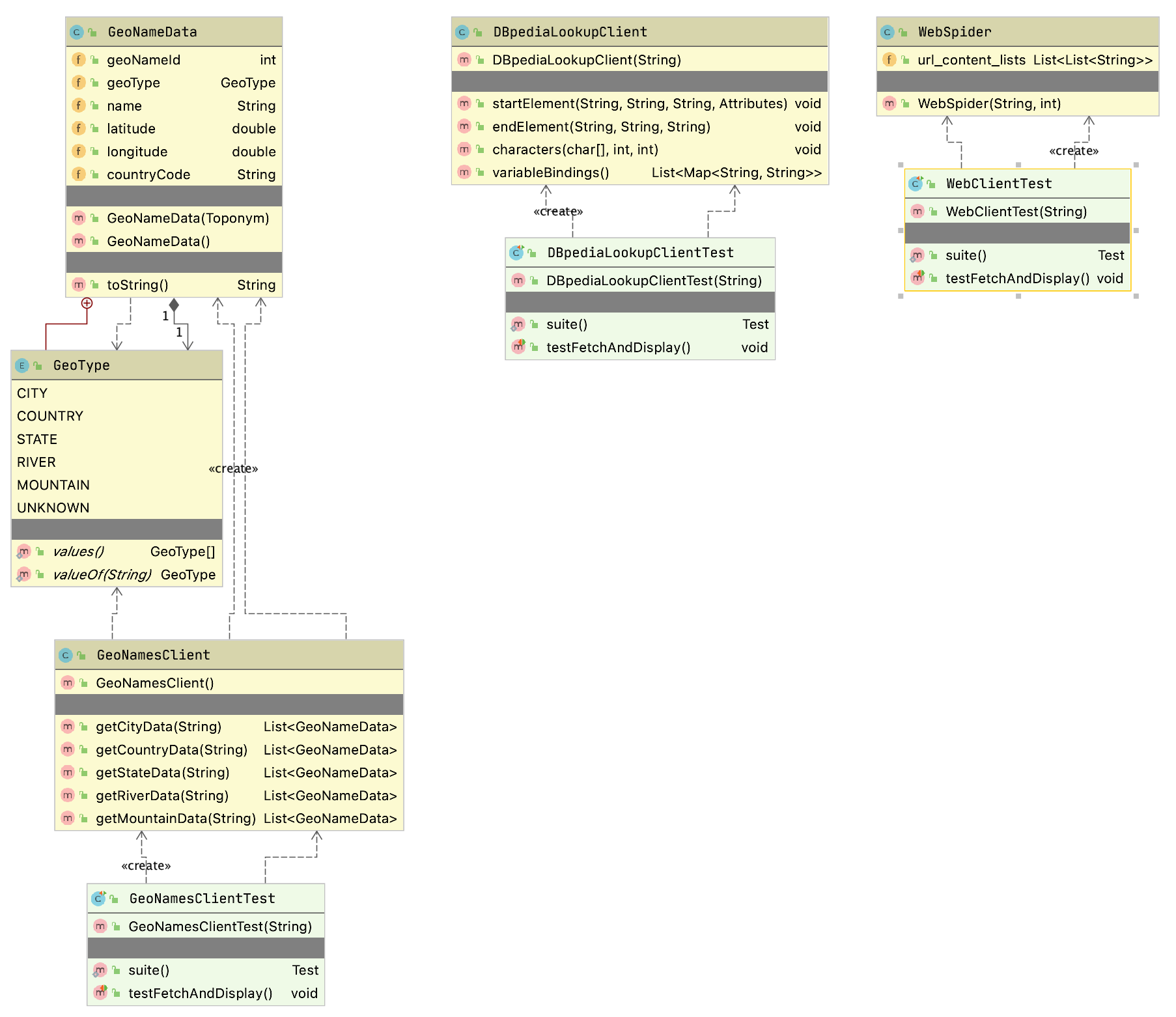
Web Scraping Examples
As a practical matter, much of the data that many people use for machine learning either comes from the web or from internal data sources. This section provides some guidance and examples for getting text data from the web.
Before we start a technical discussion about web scraping I want to point out to you that much of the information on the web is copyright and the first thing that you should do is to read the terms of service for web sites to insure that your use of “scraped” or “spidered” data conforms with the wishes of the persons or organizations who own the content and pay to run scraped web sites.
Motivation for Web Scraping
There is a huge amount of structured data available on the web via web services, semantic web/linked data markup, and APIs. That said, you will frequently find data that is useful to pull raw text from web sites but this text is usually fairly unstructured and in a messy (and frequently changing) format as web pages meant for human consumption and not meant to be ingested by software agents. In this chapter we will cover useful “web scraping” techniques. You will see that there is often a fair amount of work in dealing with different web design styles and layouts. To make things even more inconvenient you might find that your software information gathering agents will often break because of changes in web sites.
I tend to use one of three general techniques for scraping web sites. Only the first two will be covered in this chapter:
- Use an HTML parsing library that strips all HTML markup and Javascript from a page and returns a “pure text” block of text. The text in navigation menus, headers, etc. will be interspersed with what we might usually think of a “content” from a web site.
- Exploit HTML DOM (Document Object Model) formatting information on web sites to pick out headers, page titles, navigation menus, and large blocks of content text.
- Use a tool like Selenium to programatically control a web browser so your software agents can login to site and otherwise perform navigation. In other words your software agents can simulate a human using a web browser.
I seldom need to use tools like Selenium but as the saying goes “when you need them, you need them.” For simple sites I favor extracting all text as a single block and use DOM processing as needed.
I am not going to cover the use of Selenium and the Java Selenium Web-Driver APIs in this chapter because, as I mentioned, I tend to not use it frequently and I think that you are unlikely to need to do so either. I refer you to the Selenium documentation if the first two approaches in the last list do not work for your application. Selenium is primarily intended for building automating testing of complex web applications, so my occasional use in web spidering is not the common use case.
I assume that you have some experience with HTML and DOM. DOM is a tree data structure.
Web Scraping Using the Jsoup Library
We will use the MIT licensed library jsoup. One reason I selected jsoup for the examples in this chapter out of many fine libraries that provide similar functionality is the particularly nice documentation, especially The jsoup Cookbook which I urge you to bookmark as a general reference. In this chapter I will concentrate on just the most frequent web scraping use cases that I use in my own work.
The following bit of example code uses jsoup to get the text inside all P (paragraph) elements that are direct children of any DIV element. On line 14 we use the jsoup library to fetch my home web page:
 1 package com.markwatson.web_scraping;
 2
 3 import org.jsoup.*;
 4 import org.jsoup.nodes.Document;
 5 import org.jsoup.nodes.Element;
 6 import org.jsoup.select.Elements;
 7
 8 /**
 9  * Examples of using jsoup
10  */
11 public class MySitesExamples {
12
13   public static void main(String[] args) throws Exception {
14     Document doc = Jsoup.connect("https://markwatson.com")
15         .userAgent("Mozilla/5.0 (Macintosh; Intel Mac OS X 10.0; rv:77.0) Gecko/2010\
16 0101 Firefox/77.0")
17         .timeout(2000).get();
18     Elements newsHeadlines = doc.select("div p");
19     for (Element element : newsHeadlines) {
20       System.out.println(" next element text: " + element.text());
21     }
22     String all_page_text = doc.text();
23     System.out.println("All text on web page:\n" + all_page_text);
24     Elements anchors = doc.select("a[href]");
25     for (Element anchor : anchors) {
26       String uri = anchor.attr("href");
27       System.out.println(" next anchor uri: " + uri);
28       System.out.println(" next anchor text: " + anchor.text());
29     }
30     Elements absolute_uri_anchors = doc.select("a[href]");
31     for (Element anchor : absolute_uri_anchors) {
32       String uri = anchor.attr("abs:href");
33       System.out.println(" next anchor absolute uri: " + uri);
34       System.out.println(" next anchor absolute text: " + anchor.text());
35     }
36
37   }
38 }
In line 18 I am selecting the pattern that returns all P elements that are direct children of any DIV element and in lines 19-21 print the text inside these P elements.
For training data for machine learning it is useful to just grab all text on a web page and assume that common phrases dealing with web navigation, etc. will be dropped from learned models because they occur in many different training examples for different classifications. In the above listing, line 22 shows how to fetch the plain text from an entire web page. The code on line 24 fetched anchor elements and the loop in lines 25-29 prints out this anchor data as URI and text. The code in lines 30-35 does the same thing except we are converting relative URIs to absolute URIs.
Output might look like (most of the output is not shown from running this example file MySitesExamples.java):
 next element text: I am the author of 20+ books on Artificial Intelligence, Common \
Lisp, Deep Learning, Haskell, Java, Ruby, JavaScript, and the Semantic Web. I have 5\
5 US Patents.
 next element text: My customer list includes: Google, Capital One, CompassLabs, Dis\
ney, SAIC, Americast, PacBell, CastTV, Lutris Technology, Arctan Group, Sitescout.co\
m, Embed.ly, and Webmind Corporation.
All text on web page:
Mark Watson: consultant specializing in Common Lisp, deep learning and natural langu\
age processing
learning Toggle navigation Mark Watson consultant and author specializing in Common \
Lisp development and AI
 ...

 next anchor uri: #
 next anchor text: Mark Watson consultant and author specializing in Common Lisp dev\
elopment and AI research projects and commercial products
 next anchor uri: /
 next anchor text: Home page
 next anchor uri: /consulting
 next anchor text: Consulting
 next anchor uri: /blog
 next anchor text: My Blog
 next anchor uri: /books
 next anchor text: My Books
 next anchor uri: /opensource
 next anchor text: Open Source
   ...
 next anchor absolute uri: https://markwatson.com#
 next anchor absolute text: Mark Watson consultant and author specializing in Common\
 Lisp development and AI research projects and commercial products
 next anchor absolute uri: https://markwatson.com/
 next anchor absolute text: Home page
 next anchor absolute uri: https://markwatson.com/consulting
  ...
The 2gram (i.e., two words in sequence) “Toggle navigation” in the last listing has nothing to do with the real content in my site and is an artifact of using the Bootstrap CSS and Javascript tools. Often “noise” like this is simply ignored by machine learning models if it appears on many different sites but beware that this might be a problem and you might need to precisely fetch text from specific DOM elements. Similarly, notice that this last listing picks up the plain text from the navigation menus.
Notice that there are different types of URIs like #, relative, and absolute. Any characters following a # character do not affect the routing of which web page is shown (or which API is called) but the characters after the # character are available for use in specifying anchor positions on a web page or extra parameters for API calls. Relative APIs like consulting/ are understood to be relative to the base URI of the web site.
I often require that URIs be absolute URIs (i.e., starts with a protocol like “http:” or “https:”) and lines 28-33 show how to select just absolute URI anchors. In line 31 I am specifying the attribute as “abs:href” to be more selective.
## Web Spidering Using the Jericho Library
Here is another web spidering example that is different than the earlier example using the jsoup library. Here we will implement a spider using built in Java standard library network classes and also the Jericho HTML parser library.
package com.markwatson.info_spiders;

import net.htmlparser.jericho.*;

import java.io.InputStream;
import java.net.URL;
import java.net.URLConnection;
import java.util.*;

/**
 * This simple web spider returns a list of lists, each containing two strings
 * representing "URL" and "text".
 * Specifically, I do not return links on each page.
 */

/**
 * Copyright Mark Watson 2008-2020. All Rights Reserved.
 * License: Apache 2
 */

public class WebSpider {
  public WebSpider(String root_url, int max_returned_pages) throws Exception {
    String host = new URL(root_url).getHost();
    System.out.println("+ host: " + host);
    List<String> urls = new ArrayList<String>();
    Set<String> already_visited = new HashSet<String>();
    urls.add(root_url);
    int num_fetched = 0;
    while (num_fetched <= max_returned_pages && !urls.isEmpty()) {
      try {
        System.out.println("+ urls: " + urls);
        String url_str = urls.remove(0);
        System.out.println("+ url_str: " + url_str);
        if (url_str.toLowerCase().indexOf(host) > -1 &&
            !already_visited.contains(url_str)) {
          already_visited.add(url_str);
          URL url = new URL(url_str);
          URLConnection connection = url.openConnection();
          connection.setAllowUserInteraction(false);
          InputStream ins = url.openStream();
          Source source = new Source(ins);
          num_fetched++;
          TextExtractor te = new TextExtractor(source);
          String text = te.toString();
          // Skip any pages where text on page is identical to existing
          // page (e.g., http://example.com and http://exaple.com/index.html
          boolean process = true;
          for (List<String> ls : url_content_lists) {
            if (text.equals(ls.get(1))) {
              process = false;
              break;
            }
          }
          if (process) {
            try {
              Thread.sleep(500);
            } catch (Exception ignore) {
            }
            List<StartTag> anchorTags = source.getAllStartTags("a ");
            ListIterator iter = anchorTags.listIterator();
            while (iter.hasNext()) {
              StartTag anchor = (StartTag) iter.next();
              Attributes attr = anchor.parseAttributes();
              Attribute link = attr.get("href");
              String link_str = link.getValue();
              if (link_str.indexOf("http:") == -1) {
                String path = url.getPath();
                if (path.endsWith("/")) path = path.substring(0, path.length() - 1);
                int index = path.lastIndexOf("/");
                if (index > -1) path = path.substring(0, index);
                link_str = url.getHost() + "/" + path + "/" + link_str;
                link_str = "http://" + link_str.replaceAll("///", "/").replaceAll("/\
/", "/");
              }
              urls.add(link_str);
            }
            List<String> ls = new ArrayList<String>(2);
            ls.add(url_str);
            ls.add(text);
            url_content_lists.add(ls);
          }
        }
      } catch (Exception ex) {
        System.out.println("Error: " + ex);
        ex.printStackTrace();
      }
    }
  }

  public List<List<String>> url_content_lists = new ArrayList<List<String>>();
}
The test class WebClientTest shows how to use this class:
    WebSpider client = new WebSpider("http://pbs.org", 10);
    System.out.println("Found URIs: " + client.url_content_lists);
Here is the output for the test class WebClientTest:
DBPedia Entity Lookup
DBPedia contains structured data for the WikiPedia web site. In later chapters we will learn how to use the SPARQL query language to access DBPedia. Here we use a simple lookup service for any entity name. If an entity name is found in DBPedia then information on the entity is returned as an XML payload.
The implementation file is DBpediaLookupClient.java:
package com.markwatson.info_spiders;

import org.apache.http.impl.client.CloseableHttpClient;
import org.apache.http.impl.client.HttpClients;
import org.xml.sax.Attributes;
import org.xml.sax.SAXException;
import org.xml.sax.helpers.DefaultHandler;

import javax.xml.parsers.SAXParser;
import javax.xml.parsers.SAXParserFactory;
import java.util.*;

/**
 * Copyright Mark Watson 2008-2020. All Rights Reserved.
 * License: Apache-2.0
 */

// Use Georgi Kobilarov's DBpedia lookup web service
//    ref: http://lookup.dbpedia.org/api/search.asmx?op=KeywordSearch
//    example:
// http://lookup.dbpedia.org/api/search.asmx/KeywordSearch?QueryString=Flagstaff

/**
 * Searches return results that contain any of the search terms. I am going to filter
 * the results to ignore results that do not contain all search terms.
 */


public class DBpediaLookupClient extends DefaultHandler {
  public DBpediaLookupClient(String query) throws Exception {
    this.query = query;
    CloseableHttpClient client = HttpClients.createDefault();

    String query2 = query.replaceAll(" ", "+");

    SAXParserFactory factory = SAXParserFactory.newInstance();
    SAXParser sax = factory.newSAXParser();
    sax.parse(
      "http://lookup.dbpedia.org/api/search.asmx/KeywordSearch?QueryString=" +
      query2, this);

  }

  private List<Map<String, String>> variableBindings =
      new ArrayList<Map<String, String>>();
  private Map<String, String> tempBinding = null;
  private String lastElementName = null;

  public void startElement(String uri, String localName, String qName,
                           Attributes attributes) throws SAXException {
    if (qName.equalsIgnoreCase("result")) {
      tempBinding = new HashMap<String, String>();
    }
    lastElementName = qName;
  }

  public void endElement(String uri, String localName, String qName)
         throws SAXException {
    if (qName.equalsIgnoreCase("result")) {
      if (!variableBindings.contains(tempBinding) &&
           containsSearchTerms(tempBinding))
        variableBindings.add(tempBinding);
    }
  }

  public void characters(char[] ch, int start, int length) throws SAXException {
    String s = new String(ch, start, length).trim();
    if (s.length() > 0) {
      if ("Description".equals(lastElementName)) {
        if (tempBinding.get("Description") == null) {
          tempBinding.put("Description", s);
        }
        tempBinding.put("Description", "" + tempBinding.get("Description") +
                        " " + s);
      }
      if ("URI".equals(lastElementName) && s.indexOf("Category")==-1 &&
          tempBinding.get("URI") == null) {
        tempBinding.put("URI", s);
      }
      if ("Label".equals(lastElementName)) tempBinding.put("Label", s);
    }
  }

  public List<Map<String, String>> variableBindings() {
    return variableBindings;
  }
  private boolean containsSearchTerms(Map<String, String> bindings) {
    StringBuilder sb = new StringBuilder();
    for (String value : bindings.values()) sb.append(value);  // no white space
    String text = sb.toString().toLowerCase();
    StringTokenizer st = new StringTokenizer(this.query);
    while (st.hasMoreTokens()) {
      if (text.indexOf(st.nextToken().toLowerCase()) == -1) {
        return false;
      }
    }
    return true;
  }
  private String query = "";
}
The unit test class DBpediaLookupClientTest shows how to call this library:
    DBpediaLookupClient client =
        new DBpediaLookupClient("London UK");
    List<Map<String, String>> results = client.variableBindings();
    System.out.println("# query results: " + results.size());
    for (Map<String, String> map : results) {
      for (Map.Entry<String, String> entry : map.entrySet()) {
        System.out.println(entry.getKey() + " - " + entry.getValue());
      }
    }
Here is the output from this test code (with some output not shown):
# query results: 2
Description - The O2 Arena (visually typeset in branding as The O2 arena, referred t\
o as North Greenwich Arena in context of the 2012 Summer Olympics and Paralympics) i\
s a multi-purpose indoor arena located in the centre of The O2, a large entertainmen\
t complex on the Greenwich peninsula in London, England.
  ...
Label - Sports venues in London
URI - http://dbpedia.org/resource/The_O2_Arena_(London)
Description - The City of London was a United Kingdom Parliamentary constituency. It\
 was a constituency of the House of Commons of the Parliament of England then of the\
 Parliament of Great Britain from 1707 to 1800 and of the Parliament of the United K\
ingdom from 1801 to 1950. The City of London was a United Kingdom Parliamentary cons\
tituency.
  ...
Label - United Kingdom Parliamentary constituencies represented by a sitting Prime M\
inister
URI - http://dbpedia.org/resource/City_of_London_(UK_Parliament_constituency)
Client for GeoNames Service
The GeoNames service looks up information about locations. You need to [sign up for a free account])http://www.geonames.org/login) and the access key needs to be stored in an environment variable GEONAMES which is accessed in Java code using:
System.getenv("GEONAMES")
The implementation file is GeoNamesClient.java uses the utility class GeoNameData that we will look at later:
package com.markwatson.info_spiders;

import org.geonames.*;

import java.util.ArrayList;
import java.util.List;

/**
 * Copyright Mark Watson 2008-2020. All Rights Reserved.
 * License: Apache 2
 */

// You will need a free GeoNames account. Sign up:  https://www.geonames.org/login
// Then, set an environment variable: export GEONAMES=your-geonames-account-name

public class GeoNamesClient {
  public GeoNamesClient() {
  }

  private List<GeoNameData> helper(String name, String type) throws Exception {
    List<GeoNameData> ret = new ArrayList<GeoNameData>();

    String geonames_account_name = System.getenv("GEONAMES");
    if (geonames_account_name == null) {
      System.err.println("You will need a free GeoNames account.");
      System.err.println("Sign up:  https://www.geonames.org/login");
      System.err.println("Then, set an environment variable:");
      System.err.println("     export GEONAMES=your-geonames-account-name");
      throw new Exception("Need API key");
    }
    WebService.setUserName(System.getenv("GEONAMES"));

    ToponymSearchCriteria searchCriteria = new ToponymSearchCriteria();
    searchCriteria.setStyle(Style.LONG);
    searchCriteria.setQ(name);
    ToponymSearchResult searchResult = WebService.search(searchCriteria);
    for (Toponym toponym : searchResult.getToponyms()) {
      if (toponym.getFeatureClassName() != null &&
        toponym.getFeatureClassName().toString().indexOf(type) > -1 &&
        toponym.getName().indexOf(name) > -1 &&
        valid(toponym.getName())) {
        ret.add(new GeoNameData(toponym));
      }
    }
    return ret;
  }

  private boolean valid(String str) {
    if (str.contains("0")) return false;
    if (str.contains("1")) return false;
    if (str.contains("2")) return false;
    if (str.contains("3")) return false;
    if (str.contains("4")) return false;
    if (str.contains("5")) return false;
    if (str.contains("6")) return false;
    if (str.contains("7")) return false;
    if (str.contains("8")) return false;
    return !str.contains("9");
  }

  public List<GeoNameData> getCityData(String city_name) throws Exception {
    return helper(city_name, "city");
  }

  public List<GeoNameData> getCountryData(String country_name) throws Exception {
    return helper(country_name, "country");
  }

  public List<GeoNameData> getStateData(String state_name) throws Exception {
    List<GeoNameData> states = helper(state_name, "state");
    for (GeoNameData state : states) {
      state.geoType = GeoNameData.GeoType.STATE;
    }
    return states;
  }

  public List<GeoNameData> getRiverData(String river_name) throws Exception {
    return helper(river_name, "stream");
  }

  public List<GeoNameData> getMountainData(String mountain_name) throws Exception {
    return helper(mountain_name, "mountain");
  }
}
The class GeoNamesClient in the last listing uses the class GeoNameData which processes the structured data returned from the GeoNames service and provides public fields to access this information and an implementation of toString to pretty-print the data to a string:
package com.markwatson.info_spiders;

import org.geonames.Toponym;

/**
 * Copyright Mark Watson 2008-2020. All Rights Reserved.
 * License: Apache-2.0
 */
public class GeoNameData {
  public enum GeoType {
    CITY, COUNTRY, STATE, RIVER, MOUNTAIN, UNKNOWN
  }
  public int geoNameId = 0;
  public GeoType geoType = GeoType.UNKNOWN;
  public String name = "";
  public double latitude = 0;
  public double longitude = 0;
  public String countryCode = "";

  public GeoNameData(Toponym toponym) {
    geoNameId = toponym.getGeoNameId();
    latitude = toponym.getLatitude();
    longitude = toponym.getLongitude();
    name = toponym.getName();
    countryCode = toponym.getCountryCode();
    if (toponym.getFeatureClassName().startsWith("city")) geoType = GeoType.CITY;
    if (toponym.getFeatureClassName().startsWith("country"))
       geoType = GeoType.COUNTRY;
    if (toponym.getFeatureClassName().startsWith("state")) geoType = GeoType.STATE;
    if (toponym.getFeatureClassName().startsWith("stream")) geoType = GeoType.RIVER;
    if (toponym.getFeatureClassName().startsWith("mountain"))
        geoType = GeoType.MOUNTAIN;
  }

  public GeoNameData() {
  }

  public String toString() {
    return "[GeoNameData: " + name + ", type: " + geoType + ", country code: " + cou\
ntryCode +
      ", ID: " + geoNameId + ", latitude: " + latitude +
      ", longitude: " + longitude + "]";
  }
}
The test class GeoNamesClientTest shows how to use these two classes:
1     GeoNamesClient client = new GeoNamesClient();
2     System.out.println(client.getCityData("Paris"));    pause();
3     System.out.println(client.getCountryData("Canada"));   pause();
4     System.out.println(client.getStateData("California")); pause();
5     System.out.println(client.getRiverData("Amazon"));     pause();
6     System.out.println(client.getMountainData("Whitney"));
The output from this test is shown below:
 1 [[GeoNameData: Paris, type: CITY, country code: FR, ID: 2988507, latitude: 48.85341,\
 2  longitude: 2.3488], [GeoNameData: Le Touquet-Paris-Plage, type: CITY, country code:\
 3  FR, ID: 2999139, latitude: 50.52432, longitude: 1.58571], [GeoNameData: Paris, type\
 4 : CITY, country code: US, ID: 4717560, latitude: 33.66094, longitude: -95.55551], [G\
 5 eoNameData: Balneario Nuevo Paris, type: CITY, country code: UY, ID: 3441475, latitu\
 6 de: -34.85, longitude: -56.23333], [GeoNameData: Paris, type: CITY, country code: BY\
 7 , ID: 8221628, latitude: 55.15464, longitude: 27.38456], [GeoNameData: Paris, type: \
 8 CITY, country code: TG, ID: 2364431, latitude: 7.15, longitude: 1.08333]]
 9 [[GeoNameData: Canada, type: COUNTRY, country code: CA, ID: 6251999, latitude: 60.10\
10 867, longitude: -113.64258], [GeoNameData: Canada Bay, type: COUNTRY, country code: \
11 AU, ID: 7839706, latitude: -33.8659, longitude: 151.11591]]
12 [[GeoNameData: Baja California Sur, type: STATE, country code: MX, ID: 4017698, lati\
13 tude: 25.83333, longitude: -111.83333], [GeoNameData: Baja California, type: STATE, \
14 country code: MX, ID: 4017700, latitude: 30.0, longitude: -115.0], [GeoNameData: Cal\
15 ifornia, type: STATE, country code: US, ID: 5332921, latitude: 37.25022, longitude: \
16 -119.75126]]
17 [[GeoNameData: Amazon Bay, type: RIVER, country code: PG, ID: 2133985, latitude: -10\
18 .30264, longitude: 149.36313]]
19 [[GeoNameData: Mount Whitney, type: MOUNTAIN, country code: US, ID: 5409018, latitud\
20 e: 36.57849, longitude: -118.29194], [GeoNameData: Whitney Peak, type: MOUNTAIN, cou\
21 ntry code: AQ, ID: 6628058, latitude: -76.43333, longitude: -126.05], [GeoNameData: \
22 Whitney Point, type: MOUNTAIN, country code: AQ, ID: 6628059, latitude: -66.25, long\
23 itude: 110.51667], [GeoNameData: Whitney Island, type: MOUNTAIN, country code: RU, I\
24 D: 1500850, latitude: 81.01149, longitude: 60.88737], [GeoNameData: Whitney Island, \
25 type: MOUNTAIN, country code: AQ, ID: 6628055, latitude: -69.66187, longitude: -68.5\
26 0341], [GeoNameData: Whitney Meadow, type: MOUNTAIN, country code: US, ID: 5409010, \
27 latitude: 36.43216, longitude: -118.26648], [GeoNameData: Whitney Peak, type: MOUNTA\
28 IN, country code: US, ID: 5444110, latitude: 39.43276, longitude: -106.47309], [GeoN\
29 ameData: Whitney Portal, type: MOUNTAIN, country code: US, ID: 5409011, latitude: 36\
30 .58882, longitude: -118.22592], [GeoNameData: Whitney Mountain, type: MOUNTAIN, coun\
31 try code: US, ID: 4136375, latitude: 36.40146, longitude: -93.91742], [GeoNameData: \
32 Whitney Bridge Dip, type: MOUNTAIN, country code: AU, ID: 11878190, latitude: -28.61\
33 241, longitude: 153.16546], [GeoNameData: Whitney Point, type: MOUNTAIN, country cod\
34 e: US, ID: 5815920, latitude: 47.76037, longitude: -122.85127], [GeoNameData: Whitne\
35 y Pass, type: MOUNTAIN, country code: US, ID: 5409024, latitude: 36.55577, longitude\
36 : -118.2812], [GeoNameData: Whitney Island, type: MOUNTAIN, country code: CA, ID: 61\
37 81293, latitude: 58.6505, longitude: -78.71621]]
Wrap-up for Information Gathering
Access to data is an advantage large companies usually have over individuals and small organizations. That said, there is a lot of free information on the web and I hope my simple utility classes we have covered here will be of some use to you.
I respect the rights of people and organizations who put information on the web. This includes:
- Read the terms of service on web sites to make sure your your of the site’s data is compliant and also avoid accessing any one web site too frequently.
- When you access services like DBpedia and Geonames consider caching the results so that you don’t ask the service for the same information repeatedly. This is particularly important during development and testing. In a later chapter we will see how to use the Apache Derby database to cache SPARQL queries to the DBPedia service.
Resolve Entity Names to DBPedia References
As a personal research project I have collected a large data set that maps entity names (e.g., people’s names, city names, names of music groups, company names, etc.) to the DBPedia URI for each entity. I have developed libraries to use this data in Common Lisp, Haskell, and Java. Here we use the Java version of this library.
The Java library is found in the directory ner_dbpedia in the GitHub repository. The raw data for these entity to URI mappings are found in the directory ner_dbpedia/dbpedia_as_text.
This example shows the use of a standard Java and Maven packaging technique: building a JAR file that contains resource files in addition to compiled Java code. The example code reads the required data resources from the JAR file (or the temporary target directory during development). This makes the JAR file self contained when we use this example library in later chapters.
DBPedia Entities
DBPedia is the structured RDF database that is automatically created from WikiPedia info boxes. We will go into some detail on RDF data in the later chapter Semantic Web. The raw data for these entity to URI mappings is found in the directory ner_dbpedia/dbpedia_as_text files have the format (for people in this case):
If you visit any or these URIs using a web browser, for example http://dbpedia.org/page/Al_Stewart you will see the DBPedia data for the entity formatted for human reading but to be clear the primary purpose of information in DBPedia is for use by software, not humans.
There are 58953 entities defined with their DBPedia URI and the following listing shows the breakdown of number of entities by entity type by counting the number of lines in each resource file:
The URI for each entity defines a unique identifier for real world entities as well as concepts. ## Library Implementation
The following UML class diagram shows the APIs and fields for the two classes in the package com.markwatson.ner_dbpedia for this example: NerMaps and TextToDbpediaUris:

As you see in the following figure showing the IntelliJ Community Edition project for this example, there are nine text files, one for each entity type in the directory src/main/resources. Later we will look at the code required to read these files in two cases:
- During development these files are read from target/classes.
- During client application use of the JAR file (created using mvn install) these files are read as resources from the Java class loader.
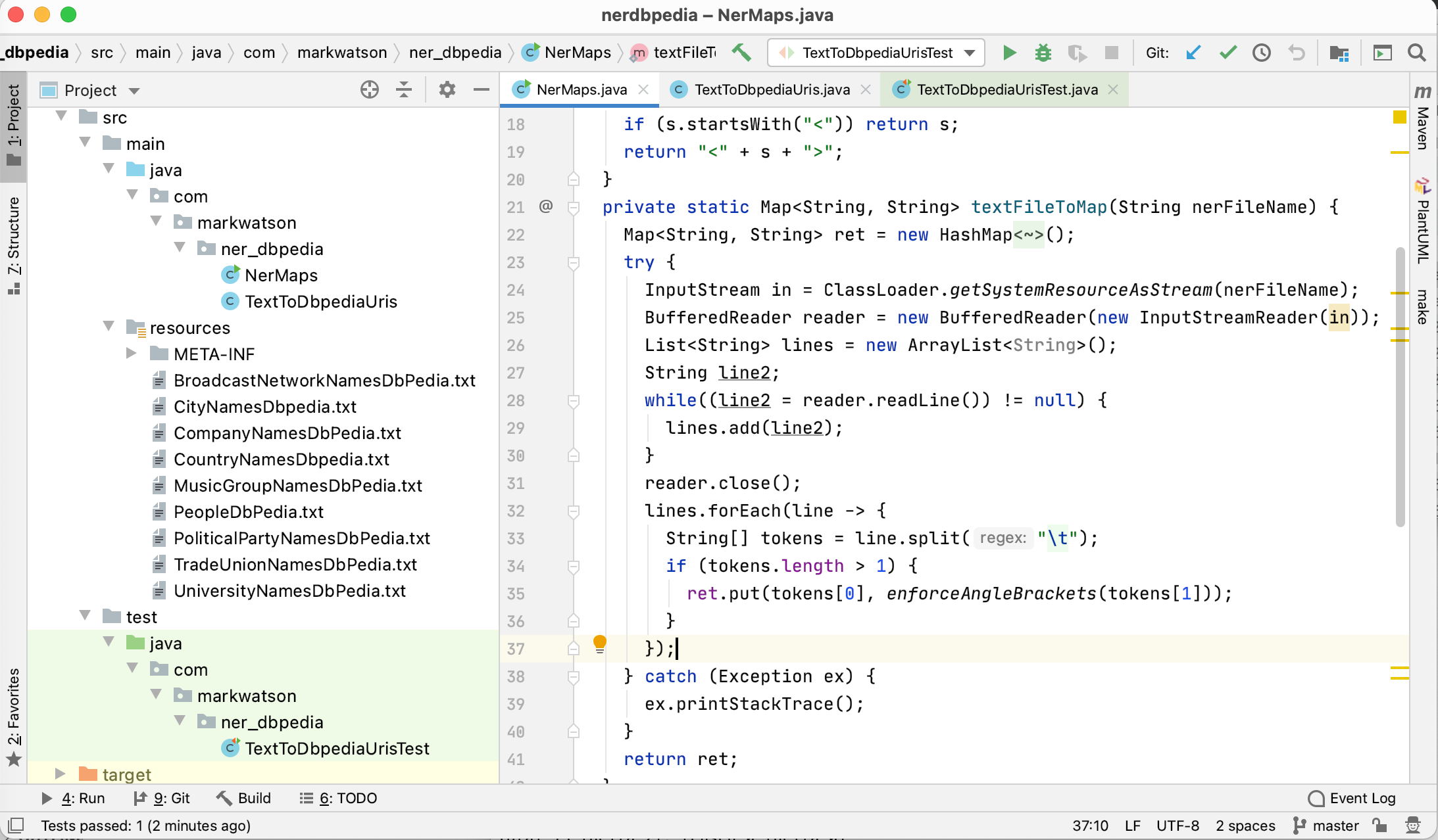
The class com.markwatson.ner_dbpedia.NerMaps is a utility for reading the raw entity mapping data files and creating hash tables for these mappings:
package com.markwatson.ner_dbpedia;

import java.io.*;
import java.nio.file.Files;
import java.nio.file.Paths;
import java.util.ArrayList;
import java.util.HashMap;
import java.util.List;
import java.util.Map;
import java.util.stream.Stream;

/**
 * Copyright Mark Watson 2020. Apache 2 license,
 */
public class NerMaps {

  private static String enforceAngleBrackets(String s) {
    if (s.startsWith("<")) return s;
    return "<" + s + ">";
  }
  private static Map<String, String> textFileToMap(String nerFileName) {
    Map<String, String> ret = new HashMap<String, String>();
    try {
      InputStream in = ClassLoader.getSystemResourceAsStream(nerFileName);
      BufferedReader reader = new BufferedReader(new InputStreamReader(in));
      List<String> lines = new ArrayList<String>();
      String line2;
      while((line2 = reader.readLine()) != null) {
        lines.add(line2);
      }
      reader.close();
      lines.forEach(line -> {
        String[] tokens = line.split("\t");
        if (tokens.length > 1) {
          ret.put(tokens[0], enforceAngleBrackets(tokens[1]));
        }
      });
    } catch (Exception ex) {
      ex.printStackTrace();
    }
    return ret;
  }

  static public final Map<String, String> broadcastNetworks =
    textFileToMap("BroadcastNetworkNamesDbPedia.txt");
  static public final Map<String, String> cityNames =
    textFileToMap("CityNamesDbpedia.txt");
  static public final Map<String, String> companyames =
    textFileToMap("CompanyNamesDbPedia.txt");
  static public final Map<String, String> countryNames =
    textFileToMap("CountryNamesDbpedia.txt");
  static public final Map<String, String> musicGroupNames =
    textFileToMap("MusicGroupNamesDbPedia.txt");
  static public final Map<String, String> personNames =
    textFileToMap("PeopleDbPedia.txt");
  static public final Map<String, String> politicalPartyNames =
    textFileToMap("PoliticalPartyNamesDbPedia.txt");
  static public final Map<String, String> tradeUnionNames =
    textFileToMap("TradeUnionNamesDbPedia.txt");
  static public final Map<String, String> universityNames =
    textFileToMap("UniversityNamesDbPedia.txt");
}
The class com.markwatson.ner_dbpedia.TextToDbpediaUris processes an input string and uses public fields to output found entity names and matching DBPedia URIs. We will use this code later in the chapter Automatically Generating Data for Knowledge Graphs.
The code in the class TextToDbpediaUris is simple and repeats two common patterns for each entity type. We will look at some of the code here.
package com.markwatson.ner_dbpedia;

import java.util.ArrayList;
import java.util.List;

public class TextToDbpediaUris {
  private TextToDbpediaUris() {
  }

  public List<String> personUris = new ArrayList<String>();
  public List<String> personNames = new ArrayList<String>();
  public List<String> companyUris = new ArrayList<String>();
  public List<String> companyNames = new ArrayList<>();
The empty constructor is private since it makes no sense to create an instance of TextToDbpediaUris without text input. The code supports nine entity types. Here we show the definition of public output fields for just two entity types (people and companies).
As a matter of programming style I generally no longer use getter and setter methods, preferring a more concise coding style. I usually make output fields package default visibility (i.e., no private or public specification so the fields are public within a package and private from other packages). Here I make them public because the package nerdbpedia developed here is meant to be used by other packages. If you prefer using getter and setter methods, modern IDEs like IntelliJ and Eclipse can generate those for you for the example code in this book.
We will handle entity names comprised of one, two, and three word sequences. We check for longer word sequences before shorter sequences:
  public TextToDbpediaUris(String text) {
    String[] tokens = tokenize(text + " . . .");
    String uri = "";
    for (int i = 0, size = tokens.length - 2; i < size; i++) {
      String n2gram = tokens[i] + " " + tokens[i + 1];
      String n3gram = n2gram + " " + tokens[i + 2];
      // check for 3grams:
      if ((uri = NerMaps.personNames.get(n3gram)) != null) {
        log("person", i, i + 2, n3gram, uri);
        i += 2;
        continue;
      }
The class NerMaps that we previously saw listed converts text files of entities to DBPedia URIs mappings to Java hash maps. The method log does two things:
- Prints out the entity type, the word indices from the original tokenized text, the entity name as a single string (combine tokens for an entity to a string), and the DBPedia URI.
- Saves entity mapping in the public fields personUris, personNames, etc.
After we check for three word entity names, we process two word names, and one word names. Here is an example:
      // check for 2grams:
      if ((s = NerMaps.personNames.get(n2gram)) != null) {
        log("person", i, i + 1, n2gram, s);
        i += 1;
        continue;
      }
The following listing shows the log method that write descriptive output and saves entity mappings. We only show the code for the entity type person:
  public void log(String nerType, int index1, int index2, String ngram, String uri) {
    System.out.println(nerType + "\t" + index1 + "\t" + index2 + "\t" +
                       ngram + "\t" + uri);
    if (!uri.startsWith("<")) uri = "<" + uri + ">";
    if (nerType.equals("person")) {
      if (!personUris.contains(uri)) {
        personUris.add(uri);
        personNames.add(ngram);
      }
    }
For some NLP applications I will use a standard tokenizer like the OpenNLP tokenizer that we used in two previous chapters. Here, I simply add spaces around punctuation characters and use the Java string split method:
  private String[] tokenize(String s) {
    return s.replaceAll("\\.", " \\. ").
             replaceAll(",", " , ").
             replaceAll("\\?", " ? ").
             replaceAll("\n", " ").
             replaceAll(";", " ; ").split(" ");
  }
The following listing shows the code snippet from the unit test code in the class TextToDbpediaUrisTest that calls the TextToDbpediaUris constructor with a text sample (junit boilerplate code is not shown):
 1 package com.markwatson.ner_dbpedia;
 2
 3   ...
 4
 5   /**
 6    * Test that is just for side effect printouts:
 7    */
 8   public void test1() throws Exception {
 9     String s = "PTL Satellite Network covered President Bill Clinton going to "
10       + " Guatemala and visiting the Coca Cola Company.";
11     TextToDbpediaUris test = new TextToDbpediaUris(s);
12   }
13 }
On line 11, the object test contains public fields for accessing the entity names and corresponding URIs. We will use these fields in the later chapters Automatically Generating Data for Knowledge Graphs and Knowledge Graph Navigator.
Here is the output from running the unit test code:
Wrap-up for Resolving Entity Names to DBPedia References
The idea behind this example is simple but useful for information processing applications using raw text input. We will use this library later in two semantic web examples.
Semantic Web
We will start with a tutorial on semantic web data standards like RDF, RDFS, and OWL, then implement a wrapper for the Apache Jena library, and finally take a deeper dive into some examples. You will learn how to do the following:
- Understand RDF data formats.
- Understand SPARQL queries for RDF data stores (both local and remote).
- Use the Apache Jena library to use local RDF data and perform SPARQL queries that return pure Java data structures.
- Use the Apache Jena library to query remote SPARQL endpoints like DBPedia and WikiData.
- Use the Apache Derby relational database to cache SPARQL remote queries for both efficiency and for building systems that may have intermittent access to the Internet.
- Take a deeper dive into RDF, RDFS, and OWL reasoners.
The semantic web is intended to provide a massive linked set of data for use by software systems just as the World Wide Web provides a massive collection of linked web pages for human reading and browsing. The semantic web is like the web in that anyone can generate any content that they want. This freedom to publish anything works for the web because we use our ability to understand natural language to interpret what we read – and often to dismiss material that based upon our own knowledge we consider to be incorrect.
Semantic web and linked data technologies are also useful for smaller amounts of data, an example being a Knowledge Graph containing information for a business. We will further explore Knowledge Graphs in the next two chapters.
The core concept for the semantic web is data integration and use from different sources. As we will soon see, the tools for implementing the semantic web are designed for encoding data and sharing data from many different sources.
I cover the semantic web in this book because I believe that semantic web technologies are complementary to AI systems for gathering and processing data on the web. As more web pages are generated by applications (as opposed to simply showing static HTML files) it becomes easier to produce both HTML for human readers and semantic data for software agents.
There are several very good semantic web toolkits for the Java language and platform. Here we use Apache Jena because it is what I often use in my own work and I believe that it is a good starting technology for your first experiments with semantic web technologies. This chapter provides an incomplete coverage of semantic web technologies and is intended as a gentle introduction to a few useful techniques and how to implement those techniques in Java. This chapter is the start of a journey in the technology that I think is as important as technologies like deep learning that get more public mindshare.
The following figure shows a layered hierarchy of data models that are used to implement semantic web applications. To design and implement these applications we need to think in terms of physical models (storage and access of RDF, RDFS, and perhaps OWL data), logical models (how we use RDF and RDFS to define relationships between data represented as unique URIs and string literals and how we logically combine data from different sources) and conceptual modeling (higher level knowledge representation and reasoning using OWL). Originally RDF data was serialized as XML data but other formats have become much more popular because they are easier to read and manually create. The top three layers in the figure might be represented as XML, or as LD-JSON (linked data JSON) or formats like N-Triples and N3 that we will use later.
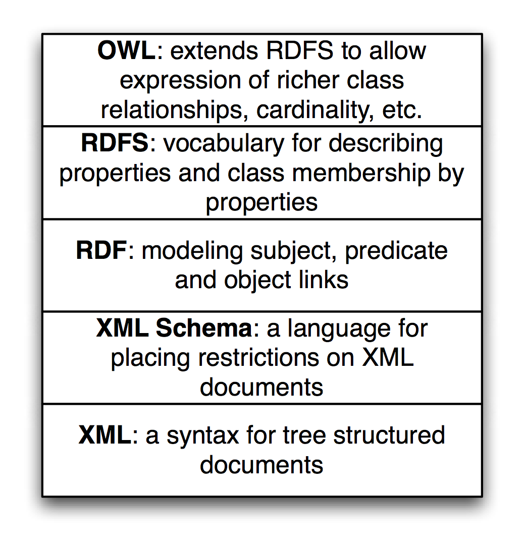
This chapter is meant to get you interested in this technology but is not intended as a complete guide. RDF data is the bedrock of the semantic web. I am also lightly covering RDFS/OWL modeling, and Descriptive Logic Reasoners which are important topics for more advanced semantic web projects.
Available Tools
In the previous edition of this book I used the open source Sesame library for the material on RDF. Sesame is now called RDF4J and is part of the Eclipse organization’s projects.
I decided to use the Apache Jena project in this new edition because I think Jena is slightly easier to set up a light weight development environment. If you need to set up an RDF server I recommend using the Fuseki server which is part of the Apache Jena project. For client applications we will use the Jena library for working with RDF and performing SPARQL queries using the example classss JenaApis that we implement later and also for querying remote SPARQL endpoints (i.e., public RDF data sources with SPARQL query interfaces) like DBPedia and WikiData.
Relational Database Model Has Problems Dealing with Rapidly Changing Data Requirements
When people are first introduced to semantic web technologies their first reaction is often something like, “I can just do that with a database.” The relational database model is an efficient way to express and work with slowly changing data schemas. There are some clever tools for dealing with data change requirements in the database world (ActiveRecord and migrations being a good example) but it is awkward to have end users and even developers tagging on new data attributes to relational database tables.
This same limitation also applies to object oriented programming and object modeling. Even with dynamic languages that facilitate modifying classes at runtime, the options for adding attributes to existing models are just too limiting. The same argument can be made against the use of XML constrained by conformance to either DTDs or XML Schemas. It is true that RDF and RDFS can be serialized to XML using many pre existing XML namespaces for different knowledge sources and schemas but it turns out that this is done in a way that does not reduce the flexibility for extending data models. XML storage is really only a serialization of RDF and many developers who are just starting to use semantic web technologies initially get confused trying to read XML serialization of RDF – almost like trying to read a PDF file with a plain text editor and something to be avoided. We will use the N-Triple and N3 formats that are simpler to read and understand.
One goal for the rest of this chapter is convincing you that modeling data with RDF and RDFS facilitates freely extending data models and also allows fairly easy integration of data from different sources using different schemas without explicitly converting data from one schema to another for reuse. You are free to add new data properties and add information to existing graphs (which we refer to a models).
RDF: The Universal Data Format
The Resource Description Framework (RDF) is used to encode information and the RDF Schema (RDFS) facilitates using data with different RDF encodings without the need to convert one set of schemas to another. Later, using OWL we can simply declare that one predicate is the same as another, that is, one predicate is a sub-predicate of another (e.g., a property containsCity can be declared to be a sub-property of containsPlace so if something contains a city then it also contains a place), etc. The predicate part of an RDF statement often refers to a property.
RDF data was originally encoded as XML and intended for automated processing. In this chapter we will use two simple to read formats called “N-Triples” and “N3.” Apache Jena can be used to convert between all RDF formats so we might as well use formats that are easier to read and understand. RDF data consists of a set of triple values:
- subject
- predicate
- object
Some of my work with semantic web technologies deals with processing news stories, extracting semantic information from the text, and storing it in RDF. I will use this application domain for the examples in this chapter and the next chapter when we implement code to automatically generate RDF for Knowledge Graphs. I deal with triples like:
- subject: a URL (or URI) of a news article.
- predicate: a relation like “containsPerson”.
- object: a literal value like “Bill Clinton” or a URI representing Bill Clinton.
In the next chapter we will use the entity recognition library we developed in an earlier chapter to create RDF from text input.
We will use either URIs or string literals as values for objects. We will always use URIs for representing subjects and predicates. In any case URIs are usually preferred to string literals. We will see an example of this preferred use but first we need to learn the N-Triple and N3 RDF formats.
I proposed the idea that RDF was more flexible than Object Modeling in programming languages, relational databases, and XML with schemas. If we can tag new attributes on the fly to existing data, how do we prevent what I might call “data chaos” as we modify existing data sources? It turns out that the solution to this problem is also the solution for encoding real semantics (or meaning) with data: we usually use unique URIs for RDF subjects, predicates, and objects, and usually with a preference for not using string literals. The definitions of predicates are tied to a namespace and later with OWL we will state the equivalence of predicates in different namespaces with the same semantic meaning. I will try to make this idea more clear with some examples and Wikipedia has a good writeup on RDF.
Any part of a triple (subject, predicate, or object) is either a URI or a string literal. URIs encode namespaces. For example, the containsPerson predicate in the last example could be written as:
http://knowledgebooks.com/ontology/#containsPerson
The first part of this URI is considered to be the namespace for this predicate “containsPerson.” When different RDF triples use this same predicate, this is some assurance to us that all users of this predicate understand to the same meaning. Furthermore, we will see later that we can use RDFS to state equivalency between this predicate (in the namespace http://knowledgebooks.com/ontology/) with predicates represented by different URIs used in other data sources. In an “artificial intelligence” sense, software that we write does not understand predicates like “containsCity”, “containsPerson”, or “isLocation” in the way that a human reader can by combining understood common meanings for the words “contains”, “city”, “is”, “person”, and “location” but for many interesting and useful types of applications that is fine as long as the predicate is used consistently. We will see shortly that we can define abbreviation prefixes for namespaces which makes RDF and RDFS files shorter and easier to read.
The Jena library supports most serialization formats for RDF:
- Turtle
- N3
- N-Triples
- NQuads
- TriG
- JSON-LD
- RDF/XML
- RDF/JSON
- TriX
- RDF Binary
A statement in N-Triple format consists of three URIs (two URIs and a string literals for the object) followed by a period to end the statement. While statements are often written one per line in a source file they can be broken across lines; it is the ending period which marks the end of a statement. The standard file extension for N-Triple format files is *.nt and the standard format for N3 format files is *.n3.
My preference is to use N-Triple format files as output from programs that I write to save data as RDF. N-Triple files don’t use any abbreviations and each RDF statement is self-contained. I often use tools like the command line commands in Jena or RDF4J to convert N-Triple files to N3 or other formats if I will be reading them or even hand editing them. Here is an example using the N3 syntax:
@prefix kb: <http://knowledgebooks.com/ontology#>
<http://news.com/201234/> kb:containsCountry "China" .
The N3 format adds prefixes (abbreviations) to the N-Triple format. In practice it would be better to use the URI http://dbpedia.org/resource/China instead of the literal value “China.”
Here we see the use of an abbreviation prefix “kb:” for the namespace for my company KnowledgeBooks.com ontologies. The first term in the RDF statement (the subject) is the URI of a news article. The second term (the predicate) is “containsCountry” in the “kb:” namespace. The last item in the statement (the object) is a string literal “China.” I would describe this RDF statement in English as, “The news article at URI http://news.com/201234 mentions the country China.”
This was a very simple N3 example which we will expand to show additional features of the N3 notation. As another example, let’s look at the case if this news article also mentions the USA. Instead of adding a whole new statement like this we can combine them using N3 notation. Here we have two separate RDF statements:
@prefix kb: <http://knowledgebooks.com/ontology#> .
<http://news.com/201234/>
kb:containsCountry
<http://dbpedia.org/resource/China> .
<http://news.com/201234/>
kb:containsCountry
<http://dbpedia.org/resource/United_States> .
We can collapse multiple RDF statements that share the same subject and optionally the same predicate:
@prefix kb: <http://knowledgebooks.com/ontology#> .
<http://news.com/201234/>
kb:containsCountry
<http://dbpedia.org/resource/China> ,
<http://dbpedia.org/resource/United_States> .
The indentation and placement on separate lines is arbitrary - use whatever style you like that is readable. We can also add in additional predicates that use the same subject (I am going to use string literals here instead of URIs for objects to make the following example more concise but in practice prefer using URIs):
@prefix kb: <http://knowledgebooks.com/ontology#> .
<http://news.com/201234/>
kb:containsCountry "China" ,
"USA" .
kb:containsOrganization "United Nations" ;
kb:containsPerson "Ban Ki-moon" , "Gordon Brown" ,
"Hu Jintao" , "George W. Bush" ,
"Pervez Musharraf" ,
"Vladimir Putin" ,
"Mahmoud Ahmadinejad" .
This single N3 statement represents ten individual RDF triples. Each section defining triples with the same subject and predicate have objects separated by commas and ending with a period. Please note that whatever RDF storage system you use (we will be using Jena) it makes no difference if we load RDF as XML, N-Triple, of N3 format files: internally subject, predicate, and object triples are stored in the same way and are used in the same way. RDF triples in a data store represent directed graphs that may not all be connected.
I promised you that the data in RDF data stores was easy to extend. As an example, let us assume that we have written software that is able to read online news articles and create RDF data that captures some of the semantics in the articles. If we extend our program to also recognize dates when the articles are published, we can simply reprocess articles and for each article add a triple to our RDF data store using a form like:
@prefix kb: <http://knowledgebooks.com/ontology#> .
<http://news.com/201234/> kb:datePublished "2008-05-11" .
Here we just represent the date as a string. We can add a type to the object representing a specific date:
@prefix xsd: <http://www.w3.org/2001/XMLSchema#> .
@prefix kb: <http://knowledgebooks.com/ontology#> .
<http://news.com/201234/> kb:datePublished "2008-05-11"^^xsd:date .
Furthermore, if we do not have dates for all news articles that is often acceptable because when constructing SPARQL queries you can match optional patterns. If for example you are looking up articles on a specific subject then some results may have a publication date attached to the results for that article and some might not. In practice RDF supports types and we would use a date type as seen in the last example, not a string. However, in designing the example programs for this chapter I decided to simplify our representation of URIs and often use string literals as simple Java strings. For many applications this isn’t a real limitation.
Extending RDF with RDF Schema
RDF Schema (RDFS) supports the definition of classes and properties based on set inclusion. In RDFS classes and properties are orthogonal. Let’s start with looking at an example using additional namespaces:
@prefix kb: <http://knowledgebooks.com/ontology#> .
@prefix rdf: <http://www.w3.org/1999/02/22-rdf-syntax-ns#>
@prefix rdfs: <http://www.w3.org/2000/01/rdf-schema#>
@prefix dbo: <http://dbpedia.org/ontology/>
<http://news.com/201234/>
kb:containsCountry
<http://dbpedia.org/resource/China> .
<http://news.com/201234/>
kb:containsCountry
<http://dbpedia.org/resource/United_States> .
<http://dbpedia.org/resource/China>
rdfs:label "China"@en,
rdf:type dbo:Place ,
rdf:type dbo:Country .
Because the semantic web is intended to be processed automatically by software systems it is encoded as RDF. There is a problem that must be solved in implementing and using the semantic web: everyone who publishes semantic web data is free to create their own RDF schemas for storing data; for example, there is usually no single standard RDF schema definition for topics like news stories and stock market data. The SKOS is a namespace containing standard schemas and the most widely used standard is schema.org. Understanding the ways of integrating different data sources using different schemas helps to understand the design decisions behind the semantic web applications. In this chapter I often use my own schemas in the knowledgebooks.com namespace for the simple examples you see here. When you build your own production systems part of the work is searching through schema.org and SKOS to use standard name spaces and schemas when possible. The use of standard schemas helps when you link internal proprietary Knowledge Graphs used in organization with public open data from sources like WikiData and DBPedia.
We will start with an example that is an extension of the example in the last section that also uses RDFS. We add a few additional RDF statements:
@prefix kb: <http://knowledgebooks.com/ontology#> .
@prefix rdfs: <http://www.w3.org/2000/01/rdf-schema#> .
kb:containsCity rdfs:subPropertyOf kb:containsPlace .
kb:containsCountry rdfs:subPropertyOf kb:containsPlace .
kb:containsState rdfs:subPropertyOf kb:containsPlace .
The last three lines declare that:
- The property containsCity is a sub-property of containsPlace.
- The property containsCountry is a sub-property of containsPlace.
- The property containsState is a sub-property of containsPlace.
Why is this useful? For at least two reasons:
- You can query an RDF data store for all triples that use property containsPlace and also match triples with properties equal to containsCity, containsCountry, or containsState. There may not even be any triples that explicitly use the property containsPlace.
- Consider a hypothetical case where you are using two different RDF data stores that use different properties for naming cities: cityName and city. You can define cityName to be a sub-property of city and then write all queries against the single property name city. This removes the necessity to convert data from different sources to use the same Schema. You can also use OWL to state property and class equivalency.
In addition to providing a vocabulary for describing properties and class membership by properties, RDFS is also used for logical inference to infer new triples, combine data from different RDF data sources, and to allow effective querying of RDF data stores. We will see examples of all of these features of RDFS when we later start using the Jena libraries to perform SPARQL queries.
The SPARQL Query Language
SPARQL is a query language used to query RDF data stores. While SPARQL may initially look like SQL, we will see that there are some important differences like support for RDFS and OWL inferencing and graph-based instead of relational matching operations. We will cover the basics of SPARQL in this section and then see more examples later when we learn how to embed Jena in Java applications, and see more examples in the last chapter Knowledge Graph Navigator.
We will use the N3 format RDF file test_data/news.n3 for the examples. I created this file automatically by spidering Reuters news stories on the news.yahoo.com web site and automatically extracting named entities from the text of the articles. We saw techniques for extracting named entities from text in earlier chapters. In this chapter we use these sample RDF files.
You have already seen snippets of this file and I list the entire file here for reference, edited to fit line width: you may find the file news.n3 easier to read if you are at your computer and open the file in a text editor so you will not be limited to what fits on a book page:
@prefix kb: <http://knowledgebooks.com/ontology#> .
@prefix rdfs: <http://www.w3.org/2000/01/rdf-schema#> .
kb:containsCity rdfs:subPropertyOf kb:containsPlace .
kb:containsCountry rdfs:subPropertyOf kb:containsPlace .
kb:containsState rdfs:subPropertyOf kb:containsPlace .
<http://yahoo.com/20080616/usa_flooding_dc_16/>
kb:containsCity "Burlington" , "Denver" ,
"St. Paul" ," Chicago" ,
"Quincy" , "CHICAGO" ,
"Iowa City" ;
kb:containsRegion "U.S. Midwest" , "Midwest" ;
kb:containsCountry "United States" , "Japan" ;
kb:containsState "Minnesota" , "Illinois" ,
"Mississippi" , "Iowa" ;
kb:containsOrganization "National Guard" ,
"U.S. Department of Agriculture" ,
"White House" ,
"Chicago Board of Trade" ,
"Department of Transportation" ;
kb:containsPerson "Dena Gray-Fisher" ,
"Donald Miller" ,
"Glenn Hollander" ,
"Rich Feltes" ,
"George W. Bush" ;
kb:containsIndustryTerm "food inflation" , "food" ,
"finance ministers" ,
"oil" .
<http://yahoo.com/78325/ts_nm/usa_politics_dc_2/>
kb:containsCity "Washington" , "Baghdad" ,
"Arlington" , "Flint" ;
kb:containsCountry "United States" ,
"Afghanistan" ,
"Iraq" ;
kb:containsState "Illinois" , "Virginia" ,
"Arizona" , "Michigan" ;
kb:containsOrganization "White House" ,
"Obama administration" ,
"Iraqi government" ;
kb:containsPerson "David Petraeus" ,
"John McCain" ,
"Hoshiyar Zebari" ,
"Barack Obama" ,
"George W. Bush" ,
"Carly Fiorina" ;
kb:containsIndustryTerm "oil prices" .
<http://yahoo.com/10944/ts_nm/worldleaders_dc_1/>
kb:containsCity "WASHINGTON" ;
kb:containsCountry "United States" , "Pakistan" ,
"Islamic Republic of Iran" ;
kb:containsState "Maryland" ;
kb:containsOrganization "University of Maryland" ,
"United Nations" ;
kb:containsPerson "Ban Ki-moon" , "Gordon Brown" ,
"Hu Jintao" , "George W. Bush" ,
"Pervez Musharraf" ,
"Vladimir Putin" ,
"Steven Kull" ,
"Mahmoud Ahmadinejad" .
<http://yahoo.com/10622/global_economy_dc_4/>
kb:containsCity "Sao Paulo" , "Kuala Lumpur" ;
kb:containsRegion "Midwest" ;
kb:containsCountry "United States" , "Britain" ,
"Saudi Arabia" , "Spain" ,
"Italy" , India" ,
""France" , "Canada" ,
"Russia" , "Germany" , "China" ,
"Japan" , "South Korea" ;
kb:containsOrganization "Federal Reserve Bank" ,
"European Union" ,
"European Central Bank" ,
"European Commission" ;
kb:containsPerson "Lee Myung-bak" , "Rajat Nag" ,
"Luiz Inacio Lula da Silva" ,
"Jeffrey Lacker" ;
kb:containsCompany "Development Bank Managing" ,
"Reuters" ,
"Richmond Federal Reserve Bank" ;
kb:containsIndustryTerm "central bank" , "food" ,
"energy costs" ,
"finance ministers" ,
"crude oil prices" ,
"oil prices" ,
"oil shock" ,
"food prices" ,
"Finance ministers" ,
"Oil prices" , "oil" .
In the following examples, we will use the main method in the class JenaApi (developed in the next section) that allows us to load multiple RDF input files and then to interactively enter SPARQL queries.
We will start with a simple SPARQL query for subjects (news article URLs) and objects (matching countries) with the value for the predicate equal to containsCountry. Variables in queries start with a question mark character and can have any names:
SELECT ?subject ?object
WHERE {
?subject
<http://knowledgebooks.com/ontology#containsCountry>
?object .
}
It is important for you to understand what is happening when we apply the last SPARQL query to our sample data. Conceptually, all the triples in the sample data are scanned, keeping the ones where the predicate part of a triple is equal to http://knowledgebooks.com/ontology#containsCountry. In practice RDF data stores supporting SPARQL queries index RDF data so a complete scan of the sample data is not required. This is analogous to relational databases where indices are created to avoid needing to perform complete scans of database tables.
In practice, when you are exploring a Knowledge Graph like DBPedia or WikiData (that are just very large collections of RDF triples), you might run a query and discover a useful or interesting entity URI in the triple store, then drill down to find out more about the entity. In a later chapter Knowledge Graph Navigator we attempt to automate this exploration process using the DBPedia data as a Knowledge Graph.
We will be using the same code to access the small example of RDF statements in our sample data as we will for accessing DBPedia or WikiData.
We can make this last query easier to read and reduce the chance of misspelling errors by using a namespace prefix:
PREFIX kb: <http://knowledgebooks.com/ontology#>
SELECT ?subject ?object
WHERE {
?subject kb:containsCountry ?object .
}
Using the command line option in the Jena wrapper example
We will later implement the Java class JenaApis. You can run the method main in the Java class JenaApis using the following to load RDF input files and interactively make SPARQL queries against the RDF data in the input files:
1 $ mvn exec:java -Dexec.mainClass="com.markwatson.semanticweb.JenaApis" \
2 -Dexec.args="data/news.n3 data/sample_news.nt"
The command line argument in line 3 starting with -Dexec.args= is one way to pass command line arguments to the method main. The backslash character at the end of line 2 is the way to continue a long command line request in bash or zsh.
Here is an interactive example of the last SPARQL example:
="com.markwatson.semanticweb.JenaApis" \
-Dexec.args="data/news.n3"
Multi-line queries are OK but don't use blank lines.
Enter a blank line to process query.
Enter a SPARQL query:
PREFIX kb: <http://knowledgebooks.com/ontology#>
SELECT ?subject ?object
WHERE {
?subject kb:containsCountry ?object .
}
[QueryResult vars:[subject, object]
Rows:
[http://news.yahoo.com/s/nm/20080616/bs_nm/global_economy_dc_4/, Russia]
[http://news.yahoo.com/s/nm/20080616/ts_nm/usa_flooding_dc_16/, Japan]
[http://news.yahoo.com/s/nm/20080616/bs_nm/global_economy_dc_4/, India]
[http://news.yahoo.com/s/nm/20080616/ts_nm/worldleaders_trust_dc_1/, United States]
[http://news.yahoo.com/s/nm/20080616/ts_nm/usa_politics_dc_2/, Afghanistan]
[http://news.yahoo.com/s/nm/20080616/bs_nm/global_economy_dc_4/, Saudi Arabia]
[http://news.yahoo.com/s/nm/20080616/bs_nm/global_economy_dc_4/, United States]
[http://news.yahoo.com/s/nm/20080616/bs_nm/global_economy_dc_4/, France]
[http://news.yahoo.com/s/nm/20080616/ts_nm/usa_politics_dc_2/, Iraq]
[http://news.yahoo.com/s/nm/20080616/ts_nm/worldleaders_trust_dc_1/, Pakistan]
[http://news.yahoo.com/s/nm/20080616/bs_nm/global_economy_dc_4/, Spain]
[http://news.yahoo.com/s/nm/20080616/bs_nm/global_economy_dc_4/, Italy]
[http://news.yahoo.com/s/nm/20080616/ts_nm/worldleaders_trust_dc_1/,
Islamic Republic of Iran]
[http://news.yahoo.com/s/nm/20080616/bs_nm/global_economy_dc_4/, Canada]
[http://news.yahoo.com/s/nm/20080616/bs_nm/global_economy_dc_4/, Britain]
[http://news.yahoo.com/s/nm/20080616/ts_nm/usa_politics_dc_2/, United States]
[http://news.yahoo.com/s/nm/20080616/bs_nm/global_economy_dc_4/, South Korea]
[http://news.yahoo.com/s/nm/20080616/bs_nm/global_economy_dc_4/, Germany]
[http://news.yahoo.com/s/nm/20080616/ts_nm/usa_flooding_dc_16/, United States]
[http://news.yahoo.com/s/nm/20080616/bs_nm/global_economy_dc_4/, China]
[http://news.yahoo.com/s/nm/20080616/bs_nm/global_economy_dc_4/, Japan]
Enter a SPARQL query:
We could have filtered on any other predicate, for instance containsPlace. Here is another example using a match against a string literal to find all articles exactly matching the text “Maryland.”
PREFIX kb: <http://knowledgebooks.com/ontology#>
SELECT ?subject WHERE { ?subject kb:containsState "Maryland" . }
The output is:
{ ?subject kb:containsState "Maryland" . }
[QueryResult vars:[subject]
Rows:
[http://news.yahoo.com/s/nm/20080616/ts_nm/worldleaders_trust_dc_1/]
We can also match partial string literals against regular expressions:
PREFIX kb: <http://knowledgebooks.com/ontology#>
SELECT ?subject ?object
WHERE {
?subject
kb:containsOrganization
?object FILTER regex(?object, "University") .
}
The output is:
{
?subject
kb:containsOrganization
?object FILTER regex(?object, "University") .
}
[QueryResult vars:[subject, object]
Rows:
[http://news.yahoo.com/s/nm/20080616/ts_nm/worldleaders_trust_dc_1/,
University of Maryland]
Prior to this last example query we only requested that the query return values for subject and predicate for triples that matched the query. However, we might want to return all triples whose subject (in this case a news article URI) is in one of the matched triples. Note that there are two matching triples, each terminated with a period:
PREFIX kb: <http://knowledgebooks.com/ontology#>
SELECT DISTINCT ?subject ?a_predicate ?an_object
WHERE {
?subject kb:containsOrganization ?object FILTER regex(?object,"University") .
?subject ?a_predicate ?an_object .
}
ORDER BY ?a_predicate ?an_object
LIMIT 10
OFFSET 5
When WHERE clauses contain more than one triple pattern to match, this is equivalent to a Boolean “and” operation. The DISTINCT clause removes duplicate results. The ORDER BY clause sorts the output in alphabetical order: in this case first by predicate (containsCity, containsCountry, etc.) and then by object. The LIMIT modifier limits the number of results returned and the OFFSET modifier sets the number of matching results to skip.
The output is:
{
?subject kb:containsOrganization ?object FILTER regex(?object,"University") .
?subject ?a_predicate ?an_object .
}
ORDER BY ?a_predicate ?an_object
LIMIT 10
OFFSET 5
[QueryResult vars:[subject, a_predicate, an_object]
Rows:
[http://news.yahoo.com/s/nm/20080616/ts_nm/worldleaders_trust_dc_1/,
http://knowledgebooks.com/ontology#containsOrganization,
University of Maryland]
[http://news.yahoo.com/s/nm/20080616/ts_nm/worldleaders_trust_dc_1/,
http://knowledgebooks.com/ontology#containsPerson, Ban Ki-moon]
[http://news.yahoo.com/s/nm/20080616/ts_nm/worldleaders_trust_dc_1/,
http://knowledgebooks.com/ontology#containsPerson, George W. Bush]
[http://news.yahoo.com/s/nm/20080616/ts_nm/worldleaders_trust_dc_1/,
http://knowledgebooks.com/ontology#containsPerson, Gordon Brown]
[http://news.yahoo.com/s/nm/20080616/ts_nm/worldleaders_trust_dc_1/,
http://knowledgebooks.com/ontology#containsPerson, Hu Jintao]
[http://news.yahoo.com/s/nm/20080616/ts_nm/worldleaders_trust_dc_1/,
http://knowledgebooks.com/ontology#containsPerson, Mahmoud Ahmadinejad]
[http://news.yahoo.com/s/nm/20080616/ts_nm/worldleaders_trust_dc_1/,
http://knowledgebooks.com/ontology#containsPerson, Pervez Musharraf]
[http://news.yahoo.com/s/nm/20080616/ts_nm/worldleaders_trust_dc_1/,
http://knowledgebooks.com/ontology#containsPerson, Steven Kull]
[http://news.yahoo.com/s/nm/20080616/ts_nm/worldleaders_trust_dc_1/,
http://knowledgebooks.com/ontology#containsPerson, Vladimir Putin]
[http://news.yahoo.com/s/nm/20080616/ts_nm/worldleaders_trust_dc_1/,
http://knowledgebooks.com/ontology#containsState, Maryland]
We are finished with our quick tutorial on using the SELECT query form. There are three other query forms that I am not covering in this chapter:
- CONSTRUCT – returns a new RDF graph of query results
- ASK – returns Boolean true or false indicating if a query matches any triples
- DESCRIBE – returns a new RDF graph containing matched resources
A common matching pattern that I don’t cover in this chapter is optional but the optional matching pattern is used in the examples in the later chapter Knowledge Graph Navigator.
Using Jena
Apache Jena is a complete Java library for developing RDF/RDFS/OWL applications and we will use it in this chapter. Other available libraries that we don’t use here include RDF4J (used to be Sesame), OWLAPI, AllegroGraph, Protege library, etc.
The following figure shows a UML diagram for the wrapper classes and interface that I wrote for Jena to make it easier for you to get started. My wrapper uses an in-memory RDF repository that supports inference, loading RDF/RDFS/OWL files, and performing both local and remote SPARQL queries. If you decide to use semantic web technologies in your development you will eventually want to use the full Jena APIs for programmatically creating new RDF triples, finer control of the type of repository (options are in-memory, disk based, and database), type definitions and inferencing, and programmatically using query results. That said, using my wrapper library is a good place for you to start experimenting.
Referring to the following figure, the class constructor JenaApis opens a new in-memory RDF triple store and supplies the public APIs we will use later. The data class QueryResults has public class variables for variable names used in a query and a list or rows, one row for each query result. The class Cache is used internally to cache SPARQL query results for later to improve performance and use without having online access a remote SPARQL endpoint like DBPedia or WikiData.
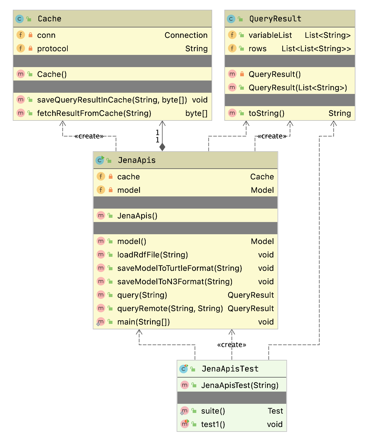
We will look in some detail at the code in this UML Class Diagram. To improve portability to alternative RDF libraries, I wrote two wrapper classes for Jena, one class to represent query results and the other to wrap the Jena APIs that I use.
The following screen shot shows the free IntelliJ Community Edition IDE used to edit one of the unit tests and run it:
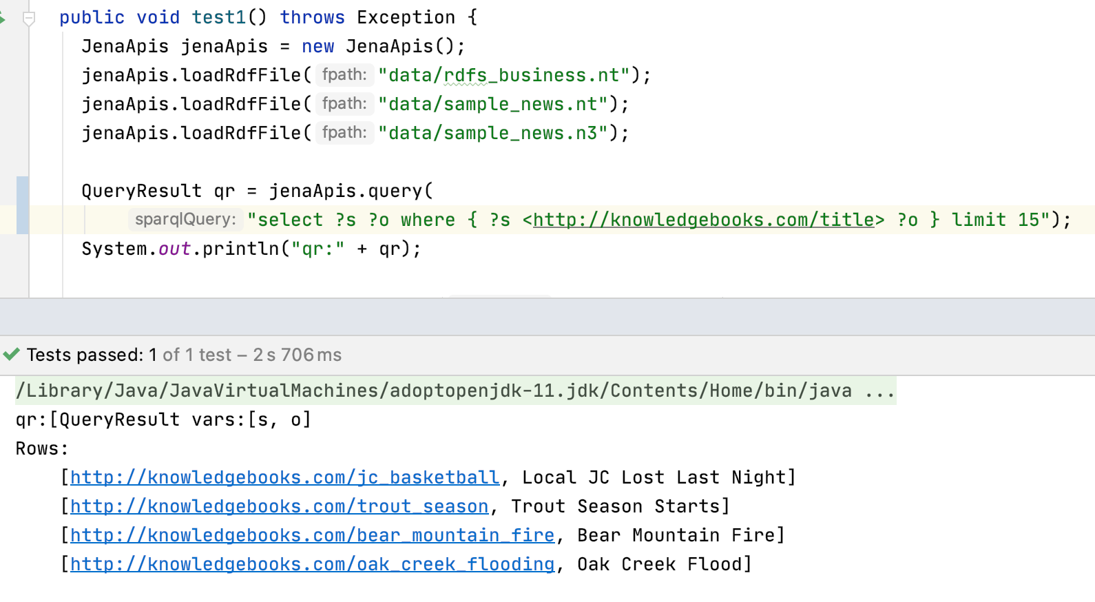
We will now look at the Java implementation of the examples for this chapter.
Java Wrapper for Jena APIs and an Example
For portability to other RDF and semantic web libraries, when we wrap the Jena APIs we want the results to be in standard Java data classes. The following listing shows the class QueryResult that contains the variables used in a SPARQL query and a list or rows containing matched value bindings for these variables:
package com.markwatson.semanticweb;
import java.io.Serializable;
import java.util.ArrayList;
import java.util.List;
public class QueryResult implements Serializable {
private QueryResult() { }
public QueryResult(List<String> variableList) {
this.variableList = variableList;
}
public List<String> variableList;
public List<List<String>> rows = new ArrayList();
public String toString() {
StringBuilder sb = new StringBuilder("[QueryResult vars:" + variableList +
"\nRows:\n");
for (List<String> row : rows) {
sb.append("\t" + row + "\n");
}
return sb.toString();
}
}
I defined a toString method so when you print an instance of the class QueryResult you see the contained data.
The following listing shows the wrapper class JenaApis:
1 package com.markwatson.semanticweb;
2
3 import org.apache.commons.lang3.SerializationUtils;
4 import org.apache.jena.query.*;
5 import org.apache.jena.rdf.model.*;
6 import org.apache.jena.riot.RDFDataMgr;
7 import org.apache.jena.riot.RDFFormat;
8
9 import java.io.FileNotFoundException;
10 import java.io.FileOutputStream;
11 import java.io.IOException;
12 import java.sql.Blob;
13 import java.sql.SQLException;
14 import java.util.ArrayList;
15 import java.util.List;
16 import java.util.Scanner;
17
18 public class JenaApis {
19
20 public JenaApis() {
21 //model = ModelFactory.createDefaultModel(); // if OWL reasoning not required
22 model = ModelFactory.createOntologyModel(); // use OWL reasoner
23 }
24
25 public Model model() {
26 return model;
27 }
28
29 public void loadRdfFile(String fpath) {
30 model.read(fpath);
31 }
32
33 public void saveModelToTurtleFormat(String outputPath) throws IOException {
34 FileOutputStream fos = new FileOutputStream(outputPath);
35 RDFDataMgr.write(fos, model, RDFFormat.TRIG_PRETTY);
36 fos.close();
37 }
38 public void saveModelToN3Format(String outputPath) throws IOException {
39 FileOutputStream fos = new FileOutputStream(outputPath);
40 RDFDataMgr.write(fos, model, RDFFormat.NTRIPLES);
41 fos.close();
42 }
43
44 public QueryResult query(String sparqlQuery) {
45 Query query = QueryFactory.create(sparqlQuery);
46 QueryExecution qexec = QueryExecutionFactory.create(query, model);
47 ResultSet results = qexec.execSelect();
48 QueryResult qr = new QueryResult(results.getResultVars());
49 for (; results.hasNext(); ) {
50 QuerySolution solution = results.nextSolution();
51 List<String> newResultRow = new ArrayList();
52 for (String var : qr.variableList) {
53 newResultRow.add(solution.get(var).toString());
54 }
55 qr.rows.add(newResultRow);
56 }
57 return qr;
58 }
59
60 public QueryResult queryRemote(String service, String sparqlQuery)
61 throws SQLException, ClassNotFoundException {
62 if (cache == null) cache = new Cache();
63 byte [] b = cache.fetchResultFromCache(sparqlQuery);
64 if (b != null) {
65 System.out.println("Found query in cache.");
66 QueryResult l = SerializationUtils.deserialize(b);
67 return l;
68 }
69 Query query = QueryFactory.create(sparqlQuery);
70 QueryExecution qexec = QueryExecutionFactory.sparqlService(service, sparqlQuery);
71 ResultSet results = qexec.execSelect();
72 QueryResult qr = new QueryResult(results.getResultVars());
73 for (; results.hasNext(); ) {
74 QuerySolution solution = results.nextSolution();
75 List<String> newResultRow = new ArrayList();
76 for (String var : qr.variableList) {
77 newResultRow.add(solution.get(var).toString());
78 }
79 qr.rows.add(newResultRow);
80 }
81 byte [] b3 = SerializationUtils.serialize(qr);
82 cache.saveQueryResultInCache(sparqlQuery, b3);
83 return qr;
84 }
85
86 private Cache cache = null;
87 private Model model;
88
89 public static void main(String[] args) {
90 /*
91 Execute using, for example:
92 mvn exec:java -Dexec.mainClass="com.markwatson.semanticweb.JenaApis" \
93 -Dexec.args="data/news.n3"
94 */
95 JenaApis ja = new JenaApis();
96 if (args.length == 0) {
97 // no RDF input file names on command line so use a default file:
98 ja.loadRdfFile("data/news.n3");
99 } else {
100 for (String fpath : args) {
101 ja.loadRdfFile(fpath);
102 }
103 }
104 System.out.println("Multi-line queries are OK but don't use blank lines.");
105 System.out.println("Enter a blank line to process query.");
106 while (true) {
107 System.out.println("Enter a SPARQL query:");
108 Scanner sc = new Scanner(System.in);
109 StringBuilder sb = new StringBuilder();
110 while (sc.hasNextLine()) { // process all inputs
111 String s = sc.nextLine();
112 if (s.equals("quit") || s.equals("QUIT") ||
113 s.equals("exit") || s.equals("EXIT"))
114 System.exit(0);
115 if (s.length() < 1) break;
116 sb.append(s);
117 sb.append("\n");
118 }
119 QueryResult qr = ja.query(sb.toString());
120 System.out.println(qr);
121 }
122 }
123 }
This code is largely self-explanatory. Line 21 or 22 should be commented out, depending on whether you want to enable OWL reasoning. In method queryRemote on line 62 we check to see if an instance of Cache has been created and if not, create one. The argument service for the method queryRemote is a SPARQL endpoint (e.g., “https://dbpedia.org/sparql”). The class QueryResult implemented Serializable so it can be converted and stored in the Derby cache database.
The method main implements a command line interface for accepting multiple lines of input. When the user enters a blank line then the previously entered non-blank lines are passed as a SPARQL local query. When run from the command line, you can enter one or more RDF input files to load prior to the SPARQL query loop.
The following class shows the unit test class JenaApisTest that provides examples for:
- Create an instance of JenaApis.
- Run a SPARQL query against the remote public DBPedia service endpoint.
- Repeat the remote SPARQL query to show query caching using the Apache Derby relational database.
- Load three input data files in N-Triple and N3 format.
- Run a SPARQL query against the RDF data that we just loaded.
- Save the current model as RDF text files in both N-Triple and N3 format.
- Making SPARQL queries that require OWL reasoning.
package com.markwatson.semanticweb;
import junit.framework.Test;
import junit.framework.TestCase;
import junit.framework.TestSuite;
public class JenaApisTest extends TestCase {
/**
* Create the test case
*
* @param testName name of the test case
*/
public JenaApisTest(String testName)
{
super( testName );
}
/**
* @return the suite of tests being tested
*/
public static Test suite()
{
return new TestSuite( JenaApisTest.class );
}
/**
* Test that is just for side effect printouts:
*/
public void test1() throws Exception {
JenaApis jenaApis = new JenaApis();
// test remote SPARQL queries against DBPedia SPARQL endpoint
QueryResult qrRemote = jenaApis.queryRemote(
"https://dbpedia.org/sparql",
"select distinct ?s { ?s ?p <http://dbpedia.org/resource/Parks> } LIMIT 10");
System.out.println("qrRemote:" + qrRemote);
System.out.println("Repeat query to test caching:");
qrRemote = jenaApis.queryRemote(
"https://dbpedia.org/sparql",
"select distinct ?s { ?s ?p <http://dbpedia.org/resource/Parks> } LIMIT 10");
System.out.println("qrRemote (hopefully from cache):" + qrRemote);
jenaApis.loadRdfFile("data/rdfs_business.nt");
jenaApis.loadRdfFile("data/sample_news.nt");
jenaApis.loadRdfFile("data/sample_news.n3");
QueryResult qr = jenaApis.query(
"select ?s ?o where { ?s <http://knowledgebooks.com/title> ?o } limit 15");
System.out.println("qr:" + qr);
jenaApis.saveModelToTurtleFormat("model_save.nt");
jenaApis.saveModelToN3Format("model_save.n3");
}
/**
* Test that is just for side effect printouts:
*/
public void testOwlReasoning() throws Exception {
JenaApis jenaApis = new JenaApis();
jenaApis.loadRdfFile("data/news.n3");
QueryResult qr = jenaApis.query(
"prefix kb: <http://knowledgebooks.com/ontology#> \n" +
"select ?s ?o where { ?s kb:containsCity ?o } ");
System.out.println("qr:" + qr);
qr = jenaApis.query(
"prefix kb: <http://knowledgebooks.com/ontology#> \n" +
"select ?s ?o where { ?s kb:containsPlace ?o }");
System.out.println("qr:" + qr);
qr = jenaApis.query( // count for each place name
"prefix kb: <http://knowledgebooks.com/ontology#> \n" +
"select ?o (count(*) as ?count) where { ?s kb:containsPlace ?o } " +
"group by ?o");
System.out.println("qr:" + qr);
}
}
To reuse the example code in this section, I recommend that you clone the entire directory semantic_web_apache_jena because it is set up for using Maven and and default logging. If you want to use the code in an existing Java project then copy the dependencies from the file pom.xml to your project. If you run mvn install then you will have a local copy installed on your system and can just install the dependency with Maven group ID com.markwatson and artifact semanticweb.
OWL: The Web Ontology Language
We have already seen a few examples of using RDFS to define sub-properties in this chapter. The Web Ontology Language (OWL) extends the expressive power of RDFS. We now look at a few OWL examples and then look at parts of the Java unit test showing three SPARQL queries that use OWL reasoning. The following RDF data stores support at least some level of OWL reasoning:
- ProtegeOwlApis - compatible with the Protege Ontology editor
- Pellet - DL reasoner
- Owlim - OWL DL reasoner compatible with some versions of Sesame
- Jena - General purpose library
- OWLAPI - a simpler API using many other libraries
- Stardog - a commercial OWL and RDF reasoning system and datastore
- Allegrograph - a commercial RDF+ and RDF reasoning system and datastore
OWL is more expressive than RDFS in that it supports cardinality, richer class relationships, and Descriptive Logic (DL) reasoning. OWL treats the idea of classes very differently than object oriented programming languages like Java and Smalltalk, but similar to the way PowerLoom (see chapter on Reasoning) uses concepts (PowerLoom’s rough equivalent to a class). In OWL, instances of a class are referred to as individuals and class membership is determined by a set of properties that allow a DL reasoner to infer class membership of an individual (this is called entailment.)
We saw an example of expressing transitive relationships when we were using PowerLoom in the chapter on Reasoning where we defined a PowerLoom rule to express that the relation “contains” is transitive. We will now look at a similar example using OWL.
We have been using the RDF file news.n3 in previous examples and we will layer new examples by adding new triples that represent RDF, RDFS, and OWL. We saw in news.n3 the definition of three triples using rdfs:subPropertyOf properties to create a more general kb:containsPlace property:
kb:containsCity rdfs:subPropertyOf kb:containsPlace .
kb:containsCountry rdfs:subPropertyOf kb:containsPlace .
kb:containsState rdfs:subPropertyOf kb:containsPlace .
kb:containsPlace rdf:type owl:transitiveProperty .
kbplace:UnitedStates kb:containsState kbplace:Illinois .
kbplace:Illinois kb:containsCity kbplace:Chicago .
We can also infer that:
kbplace:UnitedStates kb:containsPlace kbplace:Chicago .
We can also model inverse properties in OWL. For example, here we add an inverse property kb:containedIn, adding it to the example in the last listing:
kb:containedIn owl:inverseOf kb:containsPlace .
Given an RDF container that supported extended OWL DL SPARQL queries, we can now execute SPARQL queries matching the property kb:containedIn and “match” triples in the RDF triple store that have never been asserted but are inferred by the OWL reasoner.
OWL DL is a very large subset of full OWL. From reading the chapter on Reasoning and the very light coverage of OWL in this section, you should understand the concept of class membership not by explicitly stating that an object (or individual) is a member of a class, but rather because an individual has properties that can be used to infer class membership.
The World Wide Web Consortium has defined three versions of the OWL language that are in increasing order of complexity: OWL Lite, OWL DL, and OWL Full. OWL DL (supports Description Logic) is the most widely used (and recommended) version of OWL. OWL Full is not computationally decidable since it supports full logic, multiple class inheritance, and other things that probably make it computationally intractable for all but smaller problems.
We will now look at some Java code from the method testOwlReasoning in the unit test class JenaApisTest.
The following is not affected by using an OWL reasoner because the property kb:containsCity occurs directly in the input RDF data:
JenaApis jenaApis = new JenaApis();
jenaApis.loadRdfFile("data/news.n3");
QueryResult qr = jenaApis.query(
"prefix kb: <http://knowledgebooks.com/ontology#> \n" +
"select ?s ?o where { ?s kb:containsCity ?o } ");
System.out.println("qr:" + qr);
The following has been edited to keep just a few output lines per result set:
qr:[QueryResult vars:[s, o]
Rows:
[http://news.yahoo.com/s/nm/20080616/ts_nm/usa_flooding_dc_16/, St. Paul]
[http://news.yahoo.com/s/nm/20080616/ts_nm/usa_politics_dc_2/, FLINT]
[http://news.yahoo.com/s/nm/20080616/ts_nm/usa_flooding_dc_16/, CHICAGO]
... output removed. note: there were 15 results for query
[http://news.yahoo.com/s/nm/20080616/ts_nm/usa_flooding_dc_16/, Quincy]
[http://news.yahoo.com/s/nm/20080616/ts_nm/usa_flooding_dc_16/, Iowa City]
Here we use a query that is affected by using an OWL reasoner (i.e., if OWL is not enabled there will be no query results):
qr = jenaApis.query(
"prefix kb: <http://knowledgebooks.com/ontology#> \n" +
"select ?s ?o where { ?s kb:containsPlace ?o }");
System.out.println("qr:" + qr);
The code in the GitHub repo for this book is configured to use OWL by default. If you edited lines 21-22 in the file JenaApis.jav to disable OWL reasoning then revert your changes and rebuild the project.
The following has been edited to just keep a few output lines per result set:
qr:[QueryResult vars:[s, o]
Rows:
[http://news.yahoo.com/s/nm/20080616/ts_nm/usa_flooding_dc_16/, St. Paul]
[http://news.yahoo.com/s/nm/20080616/ts_nm/usa_politics_dc_2/, FLINT]
[http://news.yahoo.com/s/nm/20080616/ts_nm/usa_flooding_dc_16/, CHICAGO]
[http://news.yahoo.com/s/nm/20080616/bs_nm/global_economy_dc_4/, Kuala Lumpur]
... output removed. note: there were 46 results for query
global_economy_dc_4/, United States]
[http://news.yahoo.com/s/nm/20080616/bs_nmglobal_economy_dc_4/, Germany]
[http://news.yahoo.com/s/nm/20080616/ts_nm/usa_flooding_dc_16/, United States]
We now group (aggregate) query results and count the number of times each place name has occurred in the result (this query requires an OWL reasoner):
qr = jenaApis.query( // count for each place name
"prefix kb: <http://knowledgebooks.com/ontology#> \n" +
"select ?o (count(*) as ?count) where { ?s kb:containsPlace ?o } " +
"group by ?o");
System.out.println("qr:" + qr);
qr:[QueryResult vars:[o, count]
Rows:
[Chicago, 1^^http://www.w3.org/2001/XMLSchema#integer]
[Illinois, 2^^http://www.w3.org/2001/XMLSchema#integer]
[Arizona, 1^^http://www.w3.org/2001/XMLSchema#integer]
... output removed. note: there were 40 results for query
[United States, 4^^http://www.w3.org/2001/XMLSchema#integer]
[Iowa, 1^^http://www.w3.org/2001/XMLSchema#integer]
[Japan, 2^^http://www.w3.org/2001/XMLSchema#integer]
[Spain, 1^^http://www.w3.org/2001/XMLSchema#integer]
Note the type http://www.w3.org/2001/XMLSchema#integer using the notation for integer values bound to the variable count.
Semantic Web Wrap-up
Writing semantic web applications in Java is a very large topic, worthy of an entire book. I have covered in this chapter what for my work has been the most useful semantic web techniques: storing and querying RDF and RDFS for a specific application and using OWL when required. We will see in the next two chapters the use of RDF when automatically creating Knowledge Graphs from text data and for automatic navigation of Knowledge Graphs.
Automatically Generating Data for Knowledge Graphs
Here we develop a complete application using the package developed in the earlier chapter Resolve Entity Names to DBPedia References. The Knowledge Graph Creator (KGcreator) is a tool for automating the generation of data for Knowledge Graphs from raw text data. Here we generate RDF data for a Knowledge Graph. You might also be interested in the Knowledge Graph Creator implementation in my Common Lisp book that generates data for the Neo4J open source graph database in addition to generating RDF data.
Data created by KGcreator generates data in RDF triples suitable for loading into any linked data/semantic web data store.
This example application works by identifying entities in text. Example entity types are people, companies, country names, city names, broadcast network names, political party names, and university names. We saw earlier code for detecting entities in the chapter on making named entities to DBPedia URIs and we will reuse this code.
I originally wrote KGCreator as two research prototypes, one in Common Lisp (see my Common Lisp book) and one in Haskell. The example in this chapter is a port of these systems to Java.
Implementation Notes
The implementation is contained in a single Java class KGC and the junit test class KgcTest is used to process the test files included with this example.
As can be seen in the following figure I have defined final static strings for each type of entity type URI. For example, personTypeUri has the value http://www.w3.org/2000/01/rdf-schema#person.
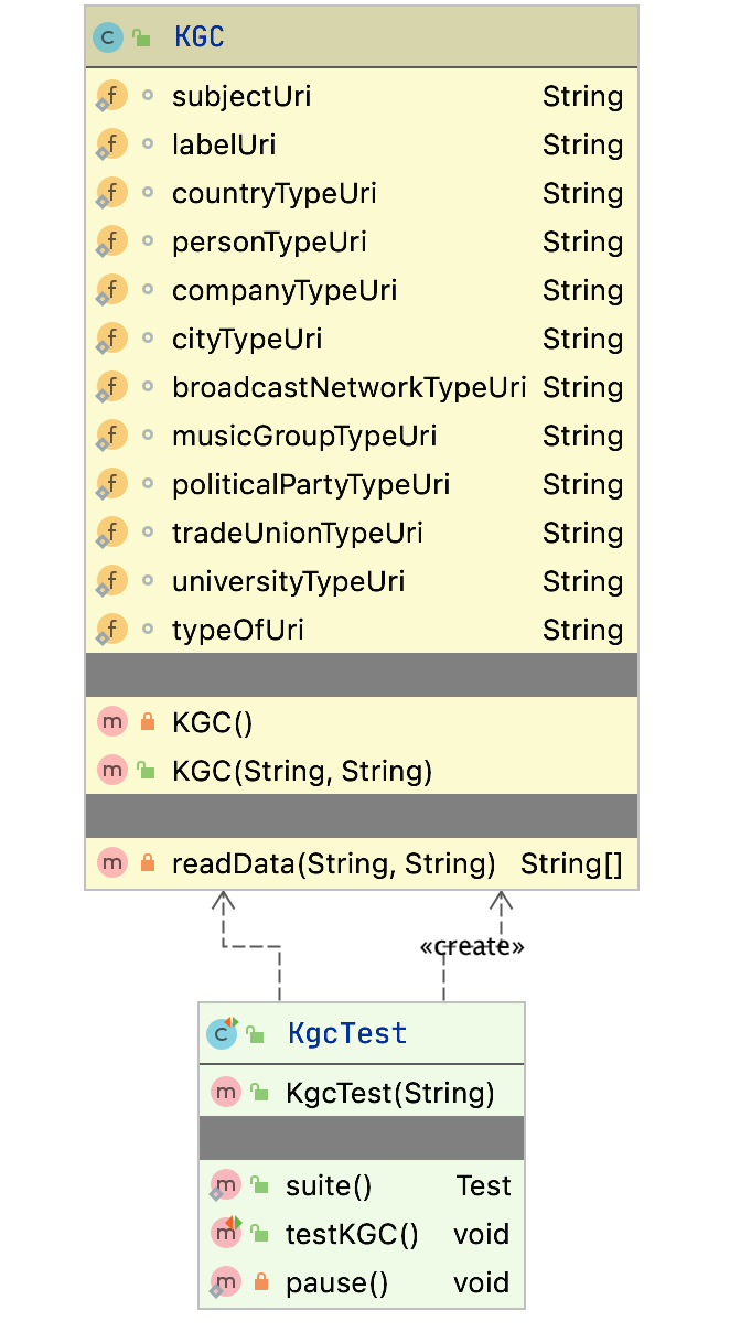
The following figure shows a screen shot of this example project in the free Community Edition of IntelliJ.

Notice in this screen shot that there are several test files in the directory test_data. The files with the file extension .meta contain a single line which is the URI for the source of the text in the matching text file. For example, the meta file test1.meta provides the URI for the source of the text in the file test1.txt.
Generating RDF Data
RDF data is comprised of triples, where the value for each triple are a subject, a predicate, and an object. Subjects are URIs, predicates are usually URIs, and objects are either literal values or URIs. Here are two triples written by this example application:
The following listing of the file KGC.java contains the implementation the main Java class for generating RDF data. Code for different entity types is similar so the following listing only shows the code for handling entity types for people and companies. The following is reformatted to fit the page width:
1 package com.knowledgegraphcreator;
2
3 import com.markwatson.ner_dbpedia.TextToDbpediaUris;
4
5 import java.io.*;
6 import java.nio.charset.StandardCharsets;
7 import java.nio.file.Files;
8 import java.nio.file.Paths;
9
10 /**
11 * Java implementation of Knowledge Graph Creator.
12 *
13 * Copyright 2020 Mark Watson. All Rights Reserved. Apache 2 license.
14 *
15 * For documentation see my book "Practical Artificial Intelligence Programming
16 * With Java", chapter "Automatically Generating Data for Knowledge Graphs"
17 * at https://leanpub.com/javaai that can be read free online.
18 *
19 */
20
21 public class KGC {
22
23 static String subjectUri =
24 "<http://www.w3.org/1999/02/22-rdf-syntax-ns#/subject>";
25 static String labelUri =
26 "<http://www.w3.org/1999/02/22-rdf-syntax-ns#/label>";
27 static String personTypeUri =
28 "<http://www.w3.org/2000/01/rdf-schema#person>";
29 static String companyTypeUri =
30 "<http://www.w3.org/2000/01/rdf-schema#company>";
31
32 static String typeOfUri =
33 "<http://www.w3.org/1999/02/22-rdf-syntax-ns#type>";
34
35 private KGC() { }
36
37 public KGC(String directoryPath, String outputRdfPath) throws IOException {
38 System.out.println("KGN");
39 PrintStream out = new PrintStream(outputRdfPath);
40 File dir = new File(directoryPath);
41 File[] directoryListing = dir.listFiles();
42 if (directoryListing != null) {
43 for (File child : directoryListing) {
44 System.out.println("child:" + child);
45 if (child.toString().endsWith(".txt")) {
46 // try to open the meta file with the same extension:
47 String metaAbsolutePath = child.getAbsolutePath();
48 File meta =
49 new File(metaAbsolutePath.substring(0,
50 metaAbsolutePath.length() - 4)
51 + ".meta");
52 System.out.println("meta:" + meta);
53 String [] text_and_meta =
54 readData(child.getAbsolutePath(), meta.getAbsolutePath());
55 String metaData = "<" + text_and_meta[1].strip() + ">";
56 TextToDbpediaUris kt =
57 new TextToDbpediaUris(text_and_meta[0]);
58 for (int i=0; i<kt.personNames.size(); i++) {
59 out.println(metaData + " " + subjectUri + " " +
60 kt.personUris.get(i) + " .");
61 out.println(kt.personUris.get(i) + " " + labelUri +
62 " \"" + kt.personNames.get(i) + "\" .");
63 out.println(kt.personUris.get(i) + " " + typeOfUri +
64 " " + personTypeUri + " .");
65 }
66 for (int i=0; i<kt.companyNames.size(); i++) {
67 out.println(metaData + " " +
68 subjectUri + " " +
69 kt.companyUris.get(i) + " .");
70 out.println(kt.companyUris.get(i) + " " +
71 labelUri + " \"" +
72 kt.companyNames.get(i) + "\" .");
73 out.println(kt.companyUris.get(i) + " " + typeOfUri +
74 " " + companyTypeUri + " .");
75 }
76 }
77 }
78 }
79 out.close();
80 }
81
82 private String [] readData(String textPath, String metaPath) throws IOException {
83 String text = Files.readString(Paths.get(textPath), StandardCharsets.UTF_8);
84 String meta = Files.readString(Paths.get(metaPath), StandardCharsets.UTF_8);
85 System.out.println("\n\n** text:\n\n" + text);
86 return new String[] { text, meta };
87 }
88 }
This code works on a list of paired files for text data and the meta data for each text file. As an example, if there is an input text file test123.txt then there would be a matching meta file test123.meta that contains the source of the data in the file test123.txt. This data source will be a URI on the web or a local file URI. The class contractor for KGC takes an output file path for writing the generated RDF data and a list of pairs of text and meta file paths.
The junit test class KgcTest will process the local directory test_data and generate an RDF output file:
1 package com.knowledgegraphcreator;
2
3 import junit.framework.Test;
4 import junit.framework.TestCase;
5 import junit.framework.TestSuite;
6
7 public class KgcTest extends TestCase {
8
9 public KgcTest(String testName) {
10 super(testName);
11 }
12
13 public static Test suite() {
14 return new TestSuite(KgcTest.class);
15 }
16
17 public void testKGC() throws Exception {
18 assertTrue(true);
19 KGC client = new KGC("test_data/", "output_with_duplicates.rdf");
20 }
21 private static void pause() {
22 try { Thread.sleep(2000);
23 } catch (Exception ignore) { }
24 }
25 }
If specific entity names occur in multiple input files there will be a few duplicated RDF statements generated. The simplest way to deal with this is to add a one line call to the awk utility to efficiently remove duplicate lines in the RDF output file. Here is a listing of the Makefile for this example:
test
echo "Removing duplicate RDF statements"
awk '!visited[$$0]++' output_with_duplicates.rdf > output.rdf
rm -f output_with_duplicates.rdf
If you are not familiar with awk and want to learn the basics then I recommend this short tutorial.
KGCreator Wrap Up
When developing applications or systems using Knowledge Graphs it is useful to be able to quickly generate test data which is the primary purpose of KGCreator. A secondary use is to generate Knowledge Graphs for production use using text data sources. In this second use case you will want to manually inspect the generated data to verify its correctness or usefulness for your application.
Knowledge Graph Navigator
The Knowledge Graph Navigator (which I will often refer to as KGN) is a tool for processing a set of entity names and automatically exploring the public Knowledge Graph DBPedia using SPARQL queries. I started to write KGN for my own use, to automate some things I used to do manually when exploring Knowledge Graphs, and later thought that KGN might be also useful for educational purposes. KGN shows the user the auto-generated SPARQL queries so hopefully the user will learn by seeing examples. KGN uses code developed in the earlier chapter Resolve Entity Names to DBPedia References and we will reuse here as well as the two Java classes JenaAPis and QueryResults (which wrap the Apache Jena library) from the chapter Semantic Web.
I have a web site devoted to different versions of KGN that you might find interesting. The most full featured version of KGN, including a full user interface, is featured in my book Loving Common Lisp, or the Savvy Programmer’s Secret Weapon that you can read free online. That version performs more speculative SPARQL queries to find information compared to the example here that I designed for ease of understanding, modification, and embedding in larger Java projects.
I chose to use DBPedia instead of WikiData for this example because DBPedia URIs are human readable. The following URIs represent the concept of a person. The semantic meanings of DBPedia and FOAF (friend of a friend) URIs are self-evident to a human reader while the WikiData URI is not:
I frequently use WikiData in my work and WikiData is one of the most useful public knowledge bases. I have both DBPedia and WikiData Sparql endpoints in the file Sparql.java that we will look at later, with the WikiData endpoint comment out. You can try manually querying WikiData at the WikiData SPARL endpoint. For example, you might explore the WikiData URI for the person concept using:
select ?p ?o where { <http://www.wikidata.org/entity/Q215627> ?p ?o } limit 10
For the rest of this chapter we will just use DBPedia.
After looking an interactive session using the example program for this chapter (that also includes listing automatically generated SPARQL queries) we will look at the implementation.
Entity Types Handled by KGN
To keep this example simple we handle just four entity types:
- People
- Companies
- Cities
- Countries
The entity detection library that we use from an earlier chapter also supports the following entity types that we don’t use here:
- Broadcast Networks
- Music Groups
- Political Parties
- Trade Unions
- Universities
In addition to finding detailed information for people, companies, cities, and countries we will also search for relationships between person entities and company entities. This search process consists of generating a series of SPARQL queries and calling the DBPedia SPARQL endpoint.
As we look at the KGN implementation I will point out where and how you can easily add support for more entity types and in the wrap-up I will suggest further projects that you might want to try implementing with this example.
General Design of KGN with Example Output
The example application works by first having the user enter names of people and companies. Using libraries written in two previous chapters, we find entities in the user’s input text, and generate SPARQL queries to DBPedia to find information about the entities and relationships between them.
We will start with looking at sample output so you have some understanding on what this implementation of KGN will and will not do. Here is the console output for the example query “Bill Gates, Melinda Gates and Steve Jobs at Apple Computer, IBM and Microsoft” (with some output removed for brevity). As you remember from the chapter Semantic Web, SPAQRL query results are expressed in class QueryResult that contains the variables (labelled as vars) in a query and a list of rows (one query result per row). Starting at line 117 in the following listing we see discovered relationships between entities in the input query.
1 Enter entities query:
2 Bill Gates, Melinda Gates and Steve Jobs at Apple Computer, IBM and Microsoft
3
4 Processing query:
5 Bill Gates, Melinda Gates and Steve Jobs at Apple Computer, IBM and Microsoft
6
7 person 0 1 Bill Gates <http://dbpedia.org/resource/Bill_Gates>
8 person 4 5 Melinda Gates <http://dbpedia.org/resource/Melinda_Gates>
9 person 7 8 Steve Jobs <http://dbpedia.org/resource/Steve_Jobs>
10 company 10 11 Apple Computer <http://dbpedia.org/resource/Apple_Inc.>
11 company 14 15 IBM <http://dbpedia.org/resource/IBM>
12 company 16 17 Microsoft <http://dbpedia.org/resource/Microsoft>
13
14 Individual People:
15
16 Bill Gates : http://dbpedia.org/resource/Bill_Gates
17 [QueryResult vars:[birthplace, label, comment, almamater, spouse]
18 Rows:
19 [http://dbpedia.org/resource/Seattle, Bill Gates, William Henry \"Bill\" Gates III\
20 (born October 28, 1955) is an American business magnate, investor, author and phila\
21 nthropist. In 1975, Gates and Paul Allen co-founded Microsoft, which became the worl\
22 d's largest PC software company. During his career at Microsoft, Gates held the posi\
23 tions of chairman, CEO and chief software architect, and was the largest individual \
24 shareholder until May 2014. Gates has authored and co-authored several books., http:\
25 //dbpedia.org/resource/Harvard_University, http://dbpedia.org/resource/Melinda_Gates\
26 ]
27
28 Melinda Gates : http://dbpedia.org/resource/Melinda_Gates
29 [QueryResult vars:[birthplace, label, comment, almamater, spouse]
30 Rows:
31 [http://dbpedia.org/resource/Dallas | http://dbpedia.org/resource/Dallas,_Texas, M\
32 elinda Gates, Melinda Ann Gates (née French; born August 15, 1964), DBE is an Americ\
33 an businesswoman and philanthropist. She is co-founder of the Bill & Melinda Gates F\
34 oundation. She worked at Microsoft, where she was project manager for Microsoft Bob,\
35 Microsoft Encarta and Expedia., http://dbpedia.org/resource/Duke_University, http:/\
36 /dbpedia.org/resource/Bill_Gates]
37
38 Steve Jobs : http://dbpedia.org/resource/Steve_Jobs
39 [QueryResult vars:[birthplace, label, comment, almamater, spouse]
40 Rows:
41 [http://dbpedia.org/resource/San_Francisco, Steve Jobs, Steven Paul \"Steve\" Jobs\
42 (/ˈdʒɒbz/; February 24, 1955 – October 5, 2011) was an American information technol\
43 ogy entrepreneur and inventor. He was the co-founder, chairman, and chief executive \
44 officer (CEO) of Apple Inc.; CEO and majority shareholder of Pixar Animation Studios\
45 ; a member of The Walt Disney Company's board of directors following its acquisition\
46 of Pixar; and founder, chairman, and CEO of NeXT Inc. Jobs is widely recognized as \
47 a pioneer of the microcomputer revolution of the 1970s and 1980s, along with Apple c\
48 o-founder Steve Wozniak. Shortly after his death, Jobs's official biographer, Walter\
49 Isaacson, described him as a \"creative entrepreneur whose passion for perfection a\
50 nd ferocious drive revolutionized six industries: personal computers, animated movie\
51 s, music, phones, tab, http://dbpedia.org/resource/Reed_College, http://dbpedia.org/\
52 resource/Laurene_Powell_Jobs]
53
54
55 Individual Companies:
56
57 Apple Computer : http://dbpedia.org/resource/Apple_Inc.
58 [QueryResult vars:[industry, netIncome, label, comment, numberOfEmployees]
59 Rows:
60 [http://dbpedia.org/resource/Computer_hardware | http://dbpedia.org/resource/Compu\
61 ter_software | http://dbpedia.org/resource/Consumer_electronics | http://dbpedia.org\
62 /resource/Corporate_Venture_Capital | http://dbpedia.org/resource/Digital_distributi\
63 on | http://dbpedia.org/resource/Fabless_manufacturing, 5.3394E10, Apple Inc., Apple\
64 Inc. is an American multinational technology company headquartered in Cupertino, Ca\
65 lifornia, that designs, develops, and sells consumer electronics, computer software,\
66 and online services. Its hardware products include the iPhone smartphone, the iPad \
67 tablet computer, the Mac personal computer, the iPod portable media player, the Appl\
68 e Watch smartwatch, and the Apple TV digital media player. Apple's consumer software\
69 includes the macOS and iOS operating systems, the iTunes media player, the Safari w\
70 eb browser, and the iLife and iWork creativity and productivity suites. Its online s\
71 ervices include the iTunes Store, the iOS App Store and Mac App Store, Apple Music, \
72 and iCloud., 115000]
73
74 IBM : http://dbpedia.org/resource/IBM
75 [QueryResult vars:[industry, netIncome, label, comment, numberOfEmployees]
76 Rows:
77 [http://dbpedia.org/resource/Cloud_computing | http://dbpedia.org/resource/Cogniti\
78 ve_computing | http://dbpedia.org/resource/Information_technology, 1.319E10, IBM, In\
79 ternational Business Machines Corporation (commonly referred to as IBM) is an Americ\
80 an multinational technology company headquartered in Armonk, New York, United States\
81 , with operations in over 170 countries. The company originated in 1911 as the Compu\
82 ting-Tabulating-Recording Company (CTR) and was renamed \"International Business Mac\
83 hines\" in 1924., 377757]
84
85 Microsoft : http://dbpedia.org/resource/Microsoft
86 [QueryResult vars:[industry, netIncome, label, comment, numberOfEmployees]
87 Rows:
88 [http://dbpedia.org/resource/Computer_hardware | http://dbpedia.org/resource/Consu\
89 mer_electronics | http://dbpedia.org/resource/Digital_distribution | http://dbpedia.\
90 org/resource/Software, , Microsoft, Microsoft Corporation /ˈmaɪkrəˌsɒft, -roʊ-, -ˌsɔ\
91 ːft/ (commonly referred to as Microsoft or MS) is an American multinational technolo\
92 gy company headquartered in Redmond, Washington, that develops, manufactures, licens\
93 es, supports and sells computer software, consumer electronics and personal computer\
94 s and services. Its best known software products are the Microsoft Windows line of o\
95 perating systems, Microsoft Office office suite, and Internet Explorer and Edge web \
96 browsers. Its flagship hardware products are the Xbox video game consoles and the Mi\
97 crosoft Surface tablet lineup. As of 2011, it was the world's largest software maker\
98 by revenue, and one of the world's most valuable companies., 114000]
99
100
101 Individual Cities:
102
103 Seattle : http://dbpedia.org/resource/Seattle
104 [QueryResult vars:[latitude_longitude, populationDensity, label, comment, country]
105 Rows:
106 [POINT(-122.33305358887 47.609722137451), 3150.979715864901, Seattle, Seattle is a\
107 West Coast seaport city and the seat of King County, Washington. With an estimated \
108 684,451 residents as of 2015, Seattle is the largest city in both the state of Washi\
109 ngton and the Pacific Northwest region of North America. As of 2015, it is estimated\
110 to be the 18th largest city in the United States. In July 2013, it was the fastest-\
111 growing major city in the United States and remained in the Top 5 in May 2015 with a\
112 n annual growth rate of 2.1%. The Seattle metropolitan area is the 15th largest metr\
113 opolitan area in the United States with over 3.7 million inhabitants. The city is si\
114 tuated on an isthmus between Puget Sound (an inlet of the Pacific Ocean) and Lake Wa\
115 shington, about 100 miles (160 km) south of the Canada–United States border. A major\
116 gateway for trade w, ]
117
118 Individual Countries:
119
120
121 Relationships between person Bill Gates person Melinda Gates:
122 [QueryResult vars:[p]
123 Rows:
124 [http://dbpedia.org/ontology/spouse]
125
126 Relationships between person Melinda Gates person Bill Gates:
127 [QueryResult vars:[p]
128 Rows:
129 [http://dbpedia.org/ontology/spouse]
130
131 Relationships between person Bill Gates company Microsoft:
132 [QueryResult vars:[p]
133 Rows:
134 [http://dbpedia.org/ontology/board]
135
136 Relationships between person Steve Jobs company Apple Computer:
137 [QueryResult vars:[p]
138 Rows:
139 [http://www.w3.org/2000/01/rdf-schema#seeAlso]
140 [http://dbpedia.org/ontology/board]
141 [http://dbpedia.org/ontology/occupation]
Since the DBPedia queries are time consuming, we use the caching layer from the earlier chapter Semantic Web when making SPARQL queries to DBPedia. The cache is especially helpful during development when the same queries are repeatedly used for testing.
The KGN user interface loop allows you to enter queries and see the results. There are two special options that you can enter instead of a query:
- sparql - this will print out all previous SPARQL queries used to present results. After entering this command the buffer of previous SPARQL queries is emptied. This option is useful for learning SPARQL and you might try pasting a few into the input field for the public DBPedia SPARQL web app and modifying them. We will use this command later in an example.
- demo - this will randomly choose a sample query.
UML Class Diagram for Example Application
The following UML Class Diagram for KGN shows you an overview of the Java classes we use and their public methods and fields.
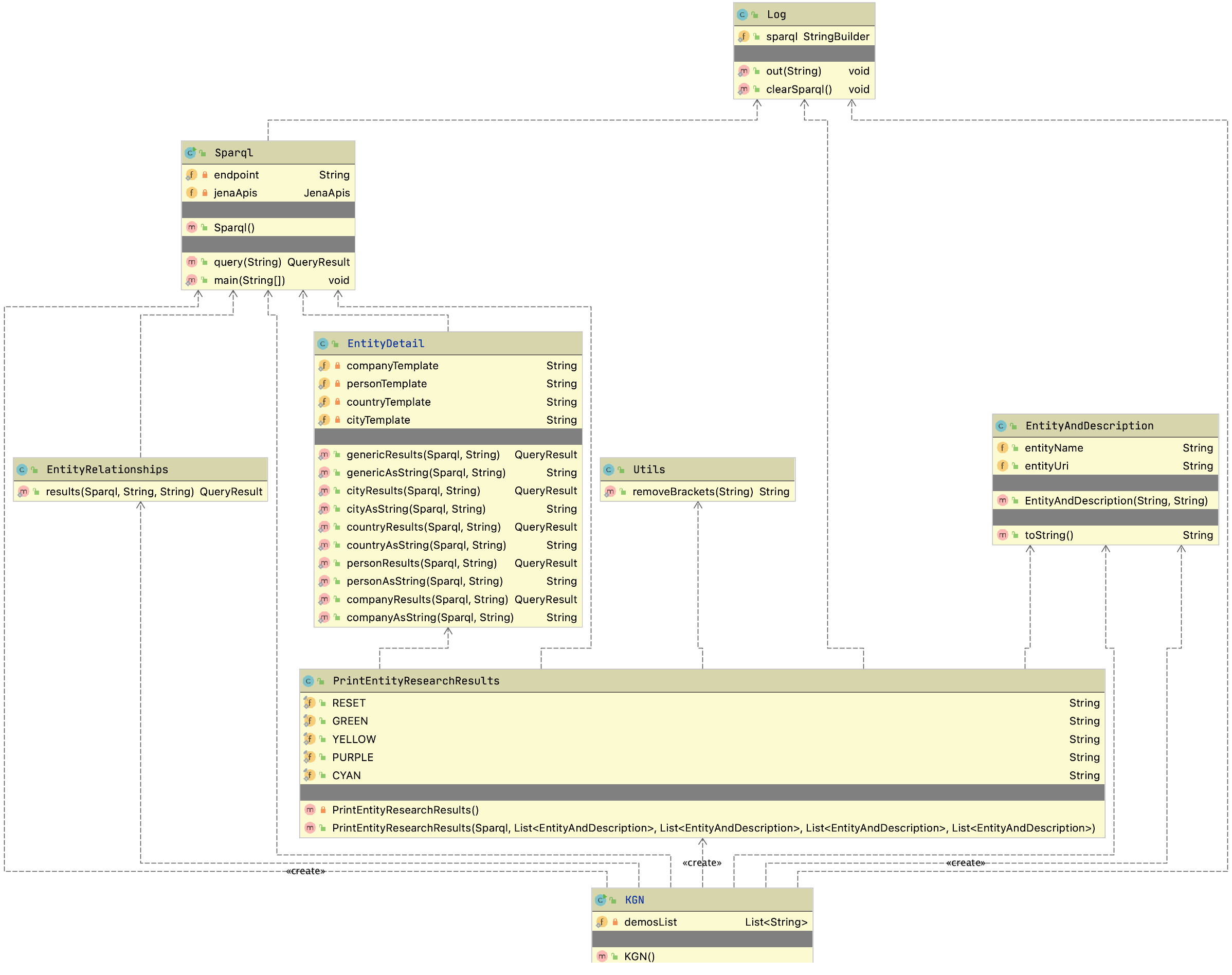
Implementation
We will walk through the classes in the UML Class Diagram for KGN in alphabetical order, the exception being that we will look at the main program in KGN.java last.
The class EntityAndDescription contains two strings, a name and a URI reference. We also override the default implementation of toString to format and display the data in an instance of this class:
1 package com.knowledgegraphnavigator;
2
3 public class EntityAndDescription {
4 public String entityName;
5 public String entityUri;
6 public EntityAndDescription(String entityName, String entityUri) {
7 this.entityName = entityName;
8 this.entityUri = entityUri;
9 }
10 public String toString() {
11 return "[EntityAndDescription name: " + entityName +
12 " description: " + entityUri + "]";
13 }
14 }
The class EntityDetail defines SPARQL query templates in lines 80-154 that have slots (using %s for string replacement) for the URI of an entity. We use different templates for different entity types. Before we look at these SPARQL query templates, let’s learn two additional features of the SPARQL language that we will need to use in these entity templates.
We mentioned the OPTIONAL triple matching patterns in the chapter Semantic Web. Before looking at the Java code, let’s first look at how optional matching works. We will run the KGN application asking for information on the city Seattle and then use the sparql command to print the generated SPARQL produced by the method cityResults (most output is not shown here for brevity). On line 2 I enter the query string “Seattle” and on line 22 I enter the command “sparql” to print out the generated SPARQL:
1 Enter entities query:
2 Seattle
3
4 Individual Cities:
5
6 Seattle : http://dbpedia.org/resource/Seattle
7 [QueryResult vars:[latitude_longitude, populationDensity, label, comment, country]
8 Rows:
9 [POINT(-122.33305358887 47.609722137451), 3150.979715864901, Seattle, Seattle is a\
10 West Coast seaport city and the seat of King County, Washington. With an estimated \
11 684,451 residents as of 2015, Seattle is the largest city in both the state of Washi\
12 ngton and the Pacific Northwest region of North America. As of 2015, it is estimated\
13 to be the 18th largest city in the United States. In July 2013, it was the fastest-\
14 growing major city in the United States and remained in the Top 5 in May 2015 with a\
15 n annual growth rate of 2.1%. The Seattle metropolitan area is the 15th largest metr\
16 opolitan area in the United States with over 3.7 million inhabitants. The city is si\
17 tuated on an isthmus between Puget Sound (an inlet of the Pacific Ocean) and Lake Wa\
18 shington, about 100 miles (160 km) south of the Canada–United States border. A major\
19 gateway for trade w, ]
20
21 Processing query:
22 sparql
23
24 Generated SPARQL used to get current results:
25
26 SELECT DISTINCT
27 (GROUP_CONCAT (DISTINCT ?latitude_longitude2; SEPARATOR=' | ')
28 AS ?latitude_longitude)
29 (GROUP_CONCAT (DISTINCT ?populationDensity2; SEPARATOR=' | ')
30 AS ?populationDensity)
31 (GROUP_CONCAT (DISTINCT ?label2; SEPARATOR=' | ') AS ?label)
32 (GROUP_CONCAT (DISTINCT ?comment2; SEPARATOR=' | ') AS ?comment)
33 (GROUP_CONCAT (DISTINCT ?country2; SEPARATOR=' | ') AS ?country) {
34 <http://dbpedia.org/resource/Seattle>
35 <http://www.w3.org/2000/01/rdf-schema#comment>
36 ?comment2 .
37 FILTER (lang(?comment2) = 'en') .
38 OPTIONAL { <http://dbpedia.org/resource/Seattle>
39 <http://www.w3.org/2003/01/geo/wgs84_pos#geometry>
40 ?latitude_longitude2 } .
41 OPTIONAL { <http://dbpedia.org/resource/Seattle>
42 <http://dbpedia.org/ontology/PopulatedPlace/populationDensity>
43 ?populationDensity2 } .
44 OPTIONAL { <http://dbpedia.org/resource/Seattle>
45 <http://dbpedia.org/ontology/country>
46 ?country2 } .
47 OPTIONAL { <http://dbpedia.org/resource/Seattle>
48 <http://www.w3.org/2000/01/rdf-schema#label>
49 ?label2 . }
50 } LIMIT 30
This listing was manually edited to fit page width. In lines 34-36, we are trying to find a triple stating which country Seattle is in. Please note that this triple matching pattern is generated as one line but I had to manually edit it here to fit the page width.
The triple matching pattern in lines 34-36 must match some triple in DBPedia or no results will be returned. In other words this matching pattern is mandatory. The four optional matching patterns in lines 38-49 specify triple patterns that may be matched. In this example there is no triple matching the following statement in the DBPedia knowledge base so the variable country2 is not bound and the query returns no results for the variable country:
<http://dbpedia.org/resource/Seattle> <http://dbpedia.org/ontology/country> ?country2
Notice also the syntax for GROUP_CONCAT used in lines 27-33, for example:
(GROUP_CONCAT (DISTINCT ?country2; SEPARATOR=' | ') AS ?country)
This collects all values assigned to the binding variable ?country2 into a string value using the separator string “ | “. Using DISTINCT with GROUP_CONCAT conveniently discards duplicate bindings for binding variables like ?country2.
Now that we have looked at SPARQL examples using OPTIONAL and GROUP_CONCAT, the templates at the end of the following listing should be easier to understand.
The methods genericResults and genericAsString in the following listing are not currently used in this example but I leave them as easy way to get information, given any entity URI. You are likely to use these if you use the code for KGN in your projects.
For each entity type, for example city, I wrote one method like cityResults that returns an instance of QueryResult calculated by using the JenaApis library from the chapter Semantic Web. For each entity type there is another method, like cityAsString that converts an instance of QueryResult to a formatted string for display.
We use the code pattern seen in lines 29-30 for each entity type. We use the static method String.format to replace occurrences of %s in the entity template string with the string representation of entity URIs.
1 package com.knowledgegraphnavigator;
2
3 import com.markwatson.semanticweb.QueryResult;
4
5 import java.sql.SQLException; // Cache layer in JenaApis library throws this
6
7 public class EntityDetail {
8
9 static public QueryResult genericResults(Sparql endpoint, String entityUri)
10 throws SQLException, ClassNotFoundException {
11 String query =
12 String.format(
13 "select distinct ?p ?o where { %s ?p ?o . " +
14 " FILTER (!regex(str(?p), 'wiki', 'i')) . " +
15 " FILTER (!regex(str(?p), 'wiki', 'i')) } limit 10",
16 entityUri);
17 return endpoint.query(query);
18 }
19
20 static public String genericAsString(Sparql endpoint, String entityUri)
21 throws SQLException, ClassNotFoundException {
22 QueryResult qr = genericResults(endpoint, entityUri);
23 return qr.toString();
24 }
25
26 static public QueryResult cityResults(Sparql endpoint, String entityUri)
27 throws SQLException, ClassNotFoundException {
28 String query =
29 String.format(cityTemplate, entityUri, entityUri, entityUri,
30 entityUri, entityUri);
31 return endpoint.query(query);
32 }
33
34 static public String cityAsString(Sparql endpoint, String entityUri)
35 throws SQLException, ClassNotFoundException {
36 QueryResult qr = cityResults(endpoint, entityUri);
37 return qr.toString();
38 }
39
40 static public QueryResult countryResults(Sparql endpoint, String entityUri)
41 throws SQLException, ClassNotFoundException {
42 String query =
43 String.format(countryTemplate, entityUri, entityUri, entityUri,
44 entityUri, entityUri);
45 return endpoint.query(query);
46 }
47
48 static public String countryAsString(Sparql endpoint, String entityUri)
49 throws SQLException, ClassNotFoundException {
50 QueryResult qr = countryResults(endpoint, entityUri);
51 return qr.toString();
52 }
53 static public QueryResult personResults(Sparql endpoint, String entityUri)
54 throws SQLException, ClassNotFoundException {
55 String query =
56 String.format(personTemplate, entityUri, entityUri, entityUri,
57 entityUri, entityUri);
58 return endpoint.query(query);
59 }
60
61 static public String personAsString(Sparql endpoint, String entityUri)
62 throws SQLException, ClassNotFoundException {
63 QueryResult qr = personResults(endpoint, entityUri);
64 return qr.toString();
65 }
66 static public QueryResult companyResults(Sparql endpoint, String entityUri)
67 throws SQLException, ClassNotFoundException {
68 String query =
69 String.format(companyTemplate, entityUri, entityUri, entityUri,
70 entityUri, entityUri);
71 return endpoint.query(query);
72 }
73
74 static public String companyAsString(Sparql endpoint, String entityUri)
75 throws SQLException, ClassNotFoundException {
76 QueryResult qr = companyResults(endpoint, entityUri);
77 return qr.toString();
78 }
79
80 static private String companyTemplate =
81 "SELECT DISTINCT" +
82 " (GROUP_CONCAT (DISTINCT ?industry2; SEPARATOR=' | ') AS ?industry)\n" +
83 " (GROUP_CONCAT (DISTINCT ?netIncome2; SEPARATOR=' | ') AS ?netIncome)\n" +
84 " (GROUP_CONCAT (DISTINCT ?label2; SEPARATOR=' | ') AS ?label)\n" +
85 " (GROUP_CONCAT (DISTINCT ?comment2; SEPARATOR=' | ') AS ?comment)\n" +
86 " (GROUP_CONCAT (DISTINCT ?numberOfEmployees2; SEPARATOR=' | ')\n" +
87 " AS ?numberOfEmployees) {\n" +
88 " %s <http://www.w3.org/2000/01/rdf-schema#comment> ?comment2 .\n" +
89 " FILTER (lang(?comment2) = 'en') .\n" +
90 " OPTIONAL { %s <http://dbpedia.org/ontology/industry> ?industry2 } .\n" +
91 " OPTIONAL { %s <http://dbpedia.org/ontology/netIncome> ?netIncome2 } .\n" +
92 " OPTIONAL {\n" +
93 " %s <http://dbpedia.org/ontology/numberOfEmployees> ?numberOfEmployees2\n" +
94 " } .\n" +
95 " OPTIONAL { %s <http://www.w3.org/2000/01/rdf-schema#label> ?label2 .\n" +
96 " FILTER (lang(?label2) = 'en') } \n" +
97 "} LIMIT 30";
98
99 static private String personTemplate =
100 "SELECT DISTINCT\n" +
101 " (GROUP_CONCAT (DISTINCT ?birthplace2; SEPARATOR=' | ') AS ?birthplace) \n"\
102 +
103 " (GROUP_CONCAT (DISTINCT ?label2; SEPARATOR=' | ') AS ?label) \n" +
104 " (GROUP_CONCAT (DISTINCT ?comment2; SEPARATOR=' | ') AS ?comment) \n" +
105 " (GROUP_CONCAT (DISTINCT ?almamater2; SEPARATOR=' | ') AS ?almamater) \n" +
106 " (GROUP_CONCAT (DISTINCT ?spouse2; SEPARATOR=' | ') AS ?spouse) { \n" +
107 " %s <http://www.w3.org/2000/01/rdf-schema#comment> ?comment2 .\n" +
108 " FILTER (lang(?comment2) = 'en') . \n" +
109 " OPTIONAL { %s <http://dbpedia.org/ontology/birthPlace> ?birthplace2 } . \n" +
110 " OPTIONAL { %s <http://dbpedia.org/ontology/almaMater> ?almamater2 } . \n" +
111 " OPTIONAL { %s <http://dbpedia.org/ontology/spouse> ?spouse2 } . \n" +
112 " OPTIONAL { %s <http://www.w3.org/2000/01/rdf-schema#label> ?label2 . \n" +
113 " FILTER (lang(?label2) = 'en') } \n" +
114 " } LIMIT 10";
115
116 static private String countryTemplate =
117 "SELECT DISTINCT" +
118 " (GROUP_CONCAT (DISTINCT ?areaTotal2; SEPARATOR=' | ') AS ?areaTotal)\n" +
119 " (GROUP_CONCAT (DISTINCT ?label2; SEPARATOR=' | ') AS ?label)\n" +
120 " (GROUP_CONCAT (DISTINCT ?comment2; SEPARATOR=' | ') AS ?comment)\n" +
121 " (GROUP_CONCAT (DISTINCT ?populationDensity2; SEPARATOR=' | ')\n" +
122 " AS ?populationDensity) {\n" +
123 " %s <http://www.w3.org/2000/01/rdf-schema#comment> ?comment2 .\n" +
124 " FILTER (lang(?comment2) = 'en') .\n" +
125 " OPTIONAL { %s <http://dbpedia.org/ontology/areaTotal> ?areaTotal2 } .\n" +
126 " OPTIONAL {\n" +
127 " %s <http://dbpedia.org/ontology/populationDensity> ?populationDensity2\n"\
128 +
129 " } .\n" +
130 " OPTIONAL { %s <http://www.w3.org/2000/01/rdf-schema#label> ?label2 . }\n" +
131 "} LIMIT 30";
132
133 static private String cityTemplate =
134 "SELECT DISTINCT\n" +
135 " (GROUP_CONCAT (DISTINCT ?latitude_longitude2; SEPARATOR=' | ') \n" +
136 " AS ?latitude_longitude) \n" +
137 " (GROUP_CONCAT (DISTINCT ?populationDensity2; SEPARATOR=' | ')\n" +
138 " AS ?populationDensity) \n" +
139 " (GROUP_CONCAT (DISTINCT ?label2; SEPARATOR=' | ') AS ?label) \n" +
140 " (GROUP_CONCAT (DISTINCT ?comment2; SEPARATOR=' | ') AS ?comment) \n" +
141 " (GROUP_CONCAT (DISTINCT ?country2; SEPARATOR=' | ') AS ?country) { \n" +
142 " %s <http://www.w3.org/2000/01/rdf-schema#comment> ?comment2 .\n" +
143 " FILTER (lang(?comment2) = 'en') . \n" +
144 " OPTIONAL {\n" +
145 " %s <http://www.w3.org/2003/01/geo/wgs84_pos#geometry>\n" +
146 " ?latitude_longitude2\n" +
147 " } . \n" +
148 " OPTIONAL {\n" +
149 " %s <http://dbpedia.org/ontology/PopulatedPlace/populationDensity>\n" +
150 " ?populationDensity2\n" +
151 " } . \n" +
152 " OPTIONAL { %s <http://dbpedia.org/ontology/country> ?country2 } . \n" +
153 " OPTIONAL { %s <http://www.w3.org/2000/01/rdf-schema#label> ?label2 . " +
154 " FILTER (lang(?label2) = 'en') } \n" +
155 "} LIMIT 30\n";
156 }
The class EntityRelationships in the next listing is used to find property relationships between two entity URIs. The RDF statement matching FILTER on line 15 prevents matching statements where the property contains the string “wiki” to avoid WikiData URI references. This class would need to be rewritten to handle, for example, the WikiData Knowledge Base instead of the DBPedia Knowledge Base. This class uses the JenaApis library developed in the chapter Semantic Web. The class Sparql that we will look at later wraps the use of the JenaApis library.
1 package com.knowledgegraphnavigator;
2
3 import com.markwatson.semanticweb.QueryResult;
4
5 import java.sql.SQLException;
6
7 public class EntityRelationships {
8
9 static public QueryResult results(Sparql endpoint,
10 String entity1Uri, String entity2Uri)
11 throws SQLException, ClassNotFoundException {
12 String query =
13 String.format(
14 "select ?p where { %s ?p %s . " +
15 " FILTER (!regex(str(?p), 'wikiPage', 'i')) } limit 10",
16 entity1Uri, entity2Uri);
17 return endpoint.query(query);
18 }
19 }
The class Log in the next listing defines a shorthand out for calling System.out.println, an instance of StringBuilder for storing all generated SPARQL queries made to DBPedia, and a utility method for clearing the stored SPARQL queries. We use the cache of SPARQL queries to support the interactive command “sparql” in the KGN application that we previously saw in an example when we saw the use of this command to display all cached SPARQL queries demonstrating the use of DISTINCT and GROUP_CONCAT.
1 package com.knowledgegraphnavigator;
2
3 public class Log {
4 static public void out(String s) { System.out.println(s); }
5 static public StringBuilder sparql = new StringBuilder();
6 static public void clearSparql() { sparql.delete(0, sparql.length()); }
7 }
The class PrintEntityResearchResults in the next listing takes results from multiple DBPedia queries, formats the results, and displays them. The class constructor has no use except for the side effect of displaying results to a user. The constructor requires the arguments:
- Sparql endpoint - we will look at the definition of class Sparql in the next section.
- List<EntityAndDescription> people - a list of person names and URIs.
- List<EntityAndDescription> companies - a list of company names and URIs.
- List<EntityAndDescription> cities - a list of city names and URIs.
- List<EntityAndDescription> countries - a list of country names and URIs.
I define static string values for a few ANSI terminal escape sequences for changing the default color of text written to a terminal. If you are running on Windows you may need to set initialization values for RESET, GREEN, YELLOW, PURPLE, and CYAN to empty strings “”.
1 package com.knowledgegraphnavigator;
2
3 import static com.knowledgegraphnavigator.Log.out;
4 import static com.knowledgegraphnavigator.Utils.removeBrackets;
5
6 import java.sql.SQLException;
7 import java.util.List;
8
9 public class PrintEntityResearchResults {
10
11 /**
12 * Note for Windows users: the Windows console may not render the following
13 * ANSI terminal escape sequences correctly. If yo have problems, just
14 * change the following to the empty string "":
15 */
16 public static final String RESET = "\u001B[0m"; // ANSI characters for styling
17 public static final String GREEN = "\u001B[32m";
18 public static final String YELLOW = "\u001B[33m";
19 public static final String PURPLE = "\u001B[35m";
20 public static final String CYAN = "\u001B[36m";
21
22 private PrintEntityResearchResults() { }
23
24 public PrintEntityResearchResults(Sparql endpoint,
25 List<EntityAndDescription> people,
26 List<EntityAndDescription> companies,
27 List<EntityAndDescription> cities,
28 List<EntityAndDescription> countries)
29 throws SQLException, ClassNotFoundException {
30 out("\n" + GREEN + "Individual People:\n" + RESET);
31 for (EntityAndDescription person : people) {
32 out(" " + GREEN + String.format("%-25s", person.entityName) +
33 PURPLE + " : " + removeBrackets(person.entityUri) + RESET);
34 out(EntityDetail.personAsString(endpoint, person.entityUri));
35 }
36 out("\n" + CYAN + "Individual Companies:\n" + RESET);
37 for (EntityAndDescription company : companies) {
38 out(" " + CYAN + String.format("%-25s", company.entityName) +
39 YELLOW + " : " + removeBrackets(company.entityUri) + RESET);
40 out(EntityDetail.companyAsString(endpoint, company.entityUri));
41 }
42 out("\n" + GREEN + "Individual Cities:\n" + RESET);
43 for (EntityAndDescription city : cities) {
44 out(" " + GREEN + String.format("%-25s", city.entityName) +
45 PURPLE + " : " + removeBrackets(city.entityUri) + RESET);
46 out(EntityDetail.cityAsString(endpoint, city.entityUri));
47 }
48 out("\n" + GREEN + "Individual Countries:\n" + RESET);
49 for (EntityAndDescription country : countries) {
50 out(" " + GREEN + String.format("%-25s", country.entityName) +
51 PURPLE + " : " + removeBrackets(country.entityUri) + RESET);
52 out(EntityDetail.countryAsString(endpoint, country.entityUri));
53 }
54 out("");
55 }
56 }
The class Sparql in the next listing wraps the JenaApis library from the chapter Semantic Web. I set the SPARQL endpoint for DBPedia on line 13. I set and commented out the WikiData SPARQL endpoint on lines 11-12. The KGN application will not work with WikiData without some modifications. If you enjoy experimenting with KGN then you might want to clone it and enable it to work simultaneously with DBPedia, WikiData, and local RDF files by using three instances of the class JenaApis.
Notice that we are importing the value of a static StringBuffer com.knowledgegraphnavigator.Log.sparql on line 5. We will use this for storing SPARQL queries for display to the user.
1 package com.knowledgegraphnavigator;
2
3 import com.markwatson.semanticweb.QueryResult;
4 import com.markwatson.semanticweb.JenaApis;
5 import static com.knowledgegraphnavigator.Log.sparql;
6 import static com.knowledgegraphnavigator.Log.out;
7
8 import java.sql.SQLException;
9
10 public class Sparql {
11 //static private String endpoint =
12 // "https://query.wikidata.org/bigdata/namespace/wdq/sparql";
13 static private String endpoint = "https://dbpedia.org/sparql";
14 public Sparql() {
15 this.jenaApis = new JenaApis();
16 }
17
18 public QueryResult query(String sparqlQuery)
19 throws SQLException, ClassNotFoundException {
20 //out(sparqlQuery); // debug for now...
21 sparql.append(sparqlQuery);
22 sparql.append(("\n\n"));
23 return jenaApis.queryRemote(endpoint, sparqlQuery);
24 }
25 private JenaApis jenaApis;
26 }
The class Utils contains one utility method removeBrackets that is used to convert a URI in SPARQL RDF statement form:
to:
The single method removeBrackets is only used in the class PrintEntityResearchResults.
1 package com.knowledgegraphnavigator;
2
3 public class Utils {
4 static public String removeBrackets(String s) {
5 if (s.startsWith("<")) return s.substring(1, s.length() - 1);
6 return s;
7 }
8 }
Finally we get to the main program implemented in the class KGN. The interactive program is implemented in the class constructor with the heart of the code being the while loop in lines 26-119 that accepts text input from the user, detects entity names and the corresponding entity types in the input text, and uses the Java classes we just looked at to find information on DBPedia for the entities in the input text as well as finding relations between these entities. Instead of entering a list of entity names the user can also enter either of the commands sparql (which we saw earlier in an example) or demo (to use a randomly chosen example query).
We use the class TextToDbpediaUris on line 38 to get the entity names and types found in the input text. You can refer back to chapter Resolve Entity Names to DBPedia References for details on using the class TextToDbpediaUris.
The loops in lines 39-70 store entity details that are displayed by calling PrintEntityResearchResults in lines 72-76. The nested loops over person entities in lines 78-91 calls EntityRelationships.results to look for relationships between two different person URIs. The same operation is done in the nested loops in lines 93-104 to find relationships between people and companies. The nested loops in lines 105-118 finds relationships between different company entities.
The static method main in lines 134-136 simply creates an instance of class KGN which has the side effect of running the example KGN program.
1 package com.knowledgegraphnavigator;
2
3 import com.markwatson.ner_dbpedia.TextToDbpediaUris;
4 import com.markwatson.semanticweb.QueryResult;
5
6 import static com.knowledgegraphnavigator.Log.out;
7 import static com.knowledgegraphnavigator.Log.sparql;
8 import static com.knowledgegraphnavigator.Log.clearSparql;
9
10 import java.util.ArrayList;
11 import java.util.Arrays;
12 import java.util.List;
13 import java.util.Scanner;
14
15 public class KGN {
16
17 private static List<String> demosList =
18 Arrays.asList(
19 "Bill Gates and Melinda Gates worked at Microsoft",
20 "IBM opened an office in Canada",
21 "Steve Jobs worked at Apple Computer and visited IBM and Microsoft in Seattle");
22
23 public KGN() throws Exception {
24 Sparql endpoint = new Sparql();
25
26 while (true) {
27 String query = getUserQueryFromConsole();
28 out("\nProcessing query:\n" + query + "\n");
29 if (query.equalsIgnoreCase("sparql")) {
30 out("Generated SPARQL used to get current results:\n");
31 out(sparql.toString());
32 out("\n");
33 clearSparql();
34 } else {
35 if (query.equalsIgnoreCase("demo")) {
36 query = demosList.get((int) (Math.random() * (demosList.size() + 1)));
37 }
38 TextToDbpediaUris kt = new TextToDbpediaUris(query);
39 List<EntityAndDescription> userSelectedPeople = new ArrayList();
40 if (kt.personNames.size() > 0) {
41 for (int i = 0; i < kt.personNames.size(); i++) {
42 userSelectedPeople.add(
43 new EntityAndDescription(kt.personNames.get(i),
44 kt.personUris.get(i)));
45 }
46 }
47 List<EntityAndDescription> userSelectedCompanies = new ArrayList();
48 if (kt.companyNames.size() > 0) {
49 for (int i = 0; i < kt.companyNames.size(); i++) {
50 userSelectedCompanies.add(
51 new EntityAndDescription(kt.companyNames.get(i),
52 kt.companyUris.get(i)));
53 }
54 }
55 List<EntityAndDescription> userSelectedCities = new ArrayList();
56 if (kt.cityNames.size() > 0) {
57 out("+++++ kt.cityNames:" + kt.cityNames.toString());
58 for (int i = 0; i < kt.cityNames.size(); i++) {
59 userSelectedCities.add(
60 new EntityAndDescription(kt.cityNames.get(i), kt.cityUris.get(i)));
61 }
62 }
63 List<EntityAndDescription> userSelectedCountries = new ArrayList();
64 if (kt.countryNames.size() > 0) {
65 out("+++++ kt.countryNames:" + kt.countryNames.toString());
66 for (int i = 0; i < kt.countryNames.size(); i++) {
67 userSelectedCountries.add(
68 new EntityAndDescription(kt.countryNames.get(i),
69 kt.countryUris.get(i)));
70 }
71 }
72 new PrintEntityResearchResults(endpoint,
73 userSelectedPeople,
74 userSelectedCompanies,
75 userSelectedCities,
76 userSelectedCountries);
77
78 for (EntityAndDescription person1 : userSelectedPeople) {
79 for (EntityAndDescription person2 : userSelectedPeople) {
80 if (person1 != person2) {
81 QueryResult qr =
82 EntityRelationships.results(endpoint, person1.entityUri,
83 person2.entityUri);
84 if (qr.rows.size() > 0) {
85 out("Relationships between person " + person1.entityName +
86 " person " + person2.entityName + ":");
87 out(qr.toString());
88 }
89 }
90 }
91 }
92
93 for (EntityAndDescription person : userSelectedPeople) {
94 for (EntityAndDescription company : userSelectedCompanies) {
95 QueryResult qr =
96 EntityRelationships.results(endpoint, person.entityUri,
97 company.entityUri);
98 if (qr.rows.size() > 0) {
99 out("Relationships between person " + person.entityName +
100 " company " + company.entityName + ":");
101 out(qr.toString());
102 }
103 }
104 }
105 for (EntityAndDescription company1 : userSelectedCompanies) {
106 for (EntityAndDescription company2 : userSelectedCompanies) {
107 if (company1 != company2) {
108 QueryResult qr =
109 EntityRelationships.results(endpoint, company1.entityUri,
110 company2.entityUri);
111 if (qr.rows.size() > 0) {
112 out("Relationships between company " + company1.entityName +
113 " company " + company2.entityName + ":");
114 out(qr.toString());
115 }
116 }
117 }
118 }
119 }
120 }
121 }
122
123 private String getUserQueryFromConsole() {
124 out("Enter entities query:");
125 Scanner input = new Scanner(System.in);
126 String ret = "";
127 while (input.hasNext()) {
128 ret = input.nextLine();
129 break;
130 }
131 return ret;
132 }
133
134 public static void main(String[] args) throws Exception {
135 new KGN();
136 }
137 }
This KGN example was hopefully both interesting to you and simple enough in its implementation (because we relied heavily on code from the last two chapters) that you feel comfortable modifying it and reusing it as a part of your own Java applications.
Wrap-up
If you enjoyed running and experimenting with this example and want to modify it for your own projects then I hope that I provided a sufficient road map for you to do so.
I suggest further projects that you might want to try implementing with this example:
- Write a web application that processes news stories and annotates them with additional data from DBPedia and/or WikiData.
- In a web or desktop application, detect entities in text and display additional information when the user’s mouse cursor hovers over a word or phrase that is identified as an entity found in DBPedia or WikiData.
- Clone this KGN example and enable it to work simultaneously with DBPedia, WikiData, and local RDF files by using three instances of the class JenaApis and in the main application loop access all three data sources.
I had the idea for the KGN application because I was spending quite a bit of time manually setting up SPARQL queries for DBPedia (and other public sources like WikiData) and I wanted to experiment with partially automating this process. I have experimented with versions of KGN written in Java, Hy language (Lisp running on Python that I wrote a short book on), Swift, and Common Lisp and all four implementations take different approaches as I experimented with different ideas. You might want to check out my web site devoted to different versions of KGN: www.knowledgegraphnavigator.com.
Conclusions
The material in this book was informed by my own work experience designing systems and writing software for artificial intelligence and information processing. If you enjoyed reading this book and you make practical use of at least some of the material I covered, then I consider my effort to be worthwhile.
Writing software is a combination of a business activity, promoting good for society, and an exploration to try out new ideas for self improvement. I believe that there is sometimes a fine line between spending too many resources tracking many new technologies versus getting stuck using old technologies at the expense of lost opportunities. My hope is that reading this book was an efficient and pleasurable use of your time, letting you try some new techniques and technologies that you had not considered before.
When we do expend resources to try new things it is almost always best to perform many small experiments and then dig deeper into areas that have a good chance of providing high value and capturing your interest.
Fail fast is a common meme but failure that we do not learn from is a waste.
I have been using the Java platform from the very beginning and although I also use many other programming languages in my work and studies, both the Java language and the Java platform provide high efficiency, scalability, many well-trained developers, and a wealth of existing infrastructure software and libraries. Investment in Java development also pays when using alternative JVM languages like JRuby, Scala, and Clojure.
If we never get to meet in person or talk on the telephone, then I would like to thank you now for taking the time to read my book.